


Simplex method
The method of the simplex was introduced by George Danzig from 1946. He is a algorithm solving linear optimization problems.
It consists in minimizing a linear function of not real variables,



where , on a set defined by means of affine (or linear) equality and inequality constraints. L'eligible set of the problem is therefore a convex polyhedron.
Method
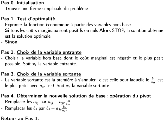
The simplex method is an iterative method traversing the vertices of the convex polyhedron until the objective function can no longer be improved. The resolution process is as follows:
- The problem is written under standard form.
- A solution is found.
- Find the pivot column.
- Find the line of the pivot and perform the Gauss method
- STOP. Optimal solution found or no solution possible.
Example resolution
Consider the following problem to apply the simplex method:
| Maximize | Z = 3x + 2y |
| under the constraints: | 2x + y ≤ 18 |
| 2x + 3y ≤ 42 | |
| 3x + y ≤ 24 | |
| x ≥ 0, y ≥ 0 |
Step 1: Write in Standard Form and Basic Solution
We transform the inequalities into equations with the addition of variables.
For this, we introduce a slack variable (x3, x4, x5) in each of the constraints of the form ≤, to transform them into equalities (see lesson on the standard form):
| 2 x1 + x2 + x3 = 18 |
| 2 x1 + 3 x2 + x4 = 42 |
| 3 x1 + x2 + x5 = 24 |
Then, we adjust the objective function to zero: Z – 3 x1 -x2 – 0 x3 – 0 x4 – 0 x5 = 0. That is to say that the variables of the canonical program are at zero, the variables of deviations are equal to the element on the right (b). From now on, it is possible to initialize the array of the simplex method.
The initial table of the simplex method is composed by all the coefficients of the original problem's decision variables and the deviation variables.
| 1st iteration | |||||||
|---|---|---|---|---|---|---|---|
| vs | 3 | 2 | |||||
| Based | Cb | b | x1 | x2 | x3 | x4 | x5 |
| x3 | 9 | 18 | 2 | 1 | 1 | 0 | 0 |
| x4 | 21 | 42 | 2 | 3 | 0 | 1 | 0 |
| x5 | 8 | 24 | 3 | 1 | 0 | 0 | 1 |
| Z | 0 | -3 | -2 | 0 | 0 | 0 |
Aside: degeneration of the simplex
A basic feasible solution is said to be degenerate if at least one of the basic variables is zero. If during the simplex algorithm, no basis encountered is degenerate, then the algorithm terminates in a finite number of iterations. If there is a degenerate base, then we can encounter a possible cycling of the algorithm: we find a base already encountered and we loop indefinitely. To deal with cases of degeneracy, we can apply Bland's rule (1977) which ensures that the algorithm stops in a finite number of iterations. When several variables are likely to enter or leave the base, we always choose the one with the smallest index.
Step 2-3: election of the input and output variable of the database
First, we establish the variable that enters the base. For this purpose, we choose the column whose value in the row Z is the lowest of all the negatives. In this case, that would be the variable x1 with a coefficient of -3. The column of the variable that enters the base, which is called pivot column (in green).
This variable is chosen because its impact on the value of Z is the greatest (greatest gradient). Entering this variable into the database consists in finding a solution in the space of solutions by following the gradient of this variable. In the following diagram, the ordinate has the greatest gradient with respect to the solution Z=0, so we will follow its axis (consider max z= xB) until you can no longer improve the solution.


Once the incoming variable has been obtained in the base, it is determined which will be the outgoing variable. The decision is made on the basis of a simple calculation: divide each independent term (column b) between the corresponding element of the pivot column, provided that both elements are strictly positive (greater than zero).
This amounts to considering that our outgoing variable will make a Gaussian pivot with the incoming variable. In other words, the incoming variable will take on a non-zero value while the outgoing variable will become zero.
We opt for the line whose result is minimal. Indeed, this calculation makes it possible to know up to what value the incoming variable can be increased. THE linear program having constraints, it is not possible to exceed the most “constraining” constraint, ie limiting the most the value of the incoming variable.
In this example: Cb: = 18/2, 42/2 and 24/3.
If there would be an element lower than or equal to zero, this quotient is not carried out. When all the elements of the pivot column are of this condition we would have fulfilled the stopping condition and the problem would have a solution without bounded part.
The term of the pivot column which had resulted in the smallest nonzero positive quotient in the previous division indicates the row of the slack variable that comes out of base. In this case, it turns out x5, with coefficient 3. This line is called line pivot (in red).
The intersection of the pivot line and the pivot column highlights the pivot element, in this case the 3.
Step 3: refresh the table
One calculates the new coefficients of the table in the following way (Gaussian pivot):
- In the pivot element row each new element is calculated as: Pivot line element = Old pivot / Pivot line element
- In the pivot column: 0 except the pivot at 1.
- In the remaining lines each element is calculated (cross product): New line element = Old line element – (Old pivot line projection *Old pivot column projection / Old pivot element).
We show the calculations for line x4 :
| Old line x4 | 42 | 2 | 3 | 0 | 1 | 0 |
| – | – | – | – | – | ||
| projection | 2*24 | 2*1 | 2*0 | 2*0 | 2*1 | |
| / | / | / | / | / | ||
| pivot | 3 | 3 | 3 | 3 | 3 | |
| = | bECOMES | = | = | = | = | |
| New line x4 | 26 | 0 | 7/3 | 0 | 1 | -2/3 |
The table corresponding to this second iteration is (note that x5 is out and that x1 has returned to its place, moreover, the objective function is no longer expressed in x1 but in x5, and its value is 24):
| Start iteration 2-th | |||||||
|---|---|---|---|---|---|---|---|
| 3 | 2 | 0 | 0 | 0 | |||
| Based | Cb | b | x1 | x2 | x3 | x4 | x5 |
| x3 | 2 | 0 | 1/3 | 1 | 0 | -2/3 | |
| x4 | 26 | 0 | 7/3 | 0 | 1 | -2/3 | |
| x1 | 8 | 1 | 1/3 | 0 | 0 | 1/3 | |
| Z | 24 | 0 | -1 | 0 | 0 | 1 |
STOP: stop conditions
If the objective is maximization, when in the last line (indicator line) there is no negative value among the costs (there is no variable with a gradient improving the solution), we obtain the stopping condition .
The value of Z (column b) is the optimal solution to the problem.
When this condition is not fulfilled, the processes are re-executed iteratively.
| 4th iteration start | |||||||
|---|---|---|---|---|---|---|---|
| 3 | 2 | 0 | 0 | 0 | |||
| Based | Cb | b | x1 | x2 | x3 | x4 | x5 |
| x2 | 0 | 12 | 0 | 1 | -1/2 | 1/2 | 0 |
| x5 | 0 | 3 | 0 | 0 | -7/4 | 1/4 | 1 |
| x1 | 0 | 3 | 1 | 0 | 3/4 | -1/4 | 0 |
| Z | 33 | 0 | 0 | 5/4 | 1/4 | 0 |
We discover that in the last line all the coefficients are positive. The optimal solution is: 33 with the solution vector (12, 3, 0, 0, 3). The solution vector is determined by the value of b on the rows of basic variables. Note that x5 = 3, i.e. the constraint 3 (containing the slack variable x5) is not saturated with 3 margin.
Abstract

Special cases
- Infinite solutions: when the simplex stops and non-basic variables have a value of 0 in the Z row, it means that there is an infinite number of solutions. To know the limits of the hyperplane (or the segment) of solutions, it suffices to recalculate the simplex by entering the variable(s) in the base.
- No solution : with the method of big M, it is possible that the definition field be empty. In this case, during the calculation of the large M certain artificial variables have a non-zero value.
- Choice of the input variable: when there is a choice among the incoming variables (same value), a basic variable of the linear program must be chosen as a priority.
- Choice of the outgoing variable: when there is a choice among the outgoing variables, the artificial variables are chosen first, then the excess variables, then the deviation variables and finally the basic variables.
- Degenerate solution: if the optimal solution has null base variables, then it is said to be degenerate, this is the case when there are more base variables than there are constraints.
Example
Note that sometimes the table is written with the value of -Z with the coefficients of c, in this case the optimal solution is obtained when all the coefficients are negative. Consider the following linear program:


First iteration:

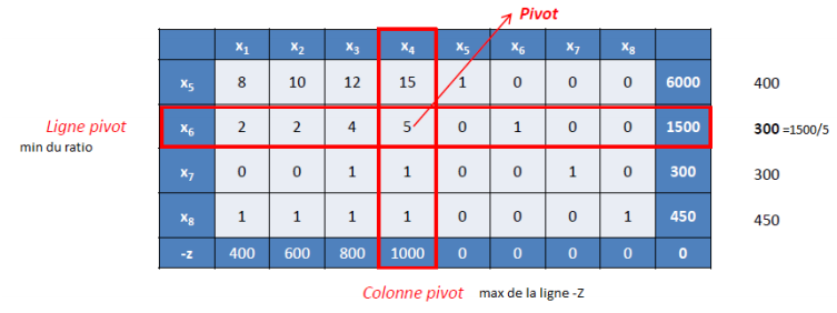
Which gives after pivot:


Here is the second iteration before and after pivot:

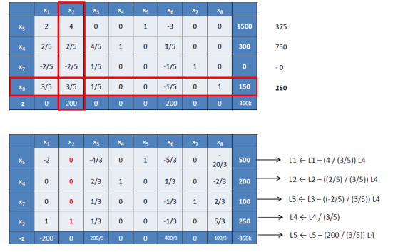
All the terms of -Z are negative, so we have an optimal solution (0, 250, 0, 200, 500, 0, 100, 0), first and third constraint are not saturated (variables of deviations at 500 and at 100); the objective function is 350000.