Simulated annealing

Contents

Annealing is a metallurgical method for obtaining crystallized solids while avoiding the glass state. Once the metal has melted, the temperature is gradually lowered until it reaches a solid state. To remove all defects, the metal is heated then cooled, in decreasing temperature stages, until it reaches a stable state.

This descending level system gave birth to the Metropolis algorithm of 1953 and then to the simulated annealing by IBM in 1983.

Presentation of the algorithm

The simulated annealing algorithm, or simulated annealing for English speakers, is therefore the adaptation algorithmic of the annealing process.

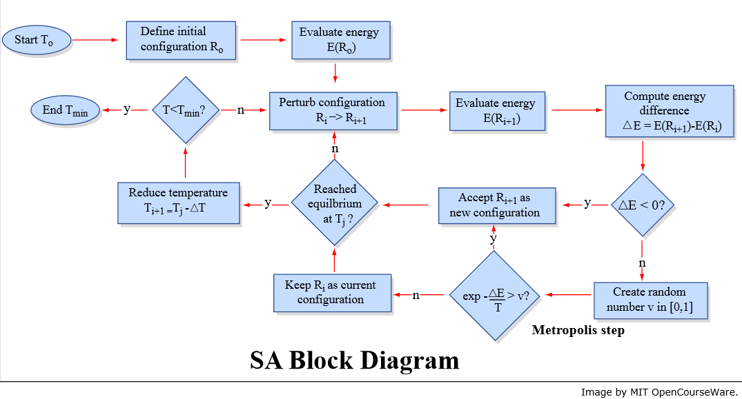
The goal is to reach a stable state of the objective function – a local or global optimum – from a random solution. This state is reached in stages, where the acceptance of a mutation is based on the "temperature" of the stage.

The simulated annealing algorithm successively generates configurations from an initial solution R₀ and an initial temperature T₀ decreasing with each iteration, until obtaining a stable configuration. The probability of accepting a new configuration is (Metropolis rule):

1 if the configuration improves the objective function;
exp (diff (E) / T) with diff (E) the energy difference and T the temperature; the energy difference is an internal function, depending on the objective function.

Algorithm flow

The annealing algorithm is as follows:

Take an initial solution R = R₀ and an initial temperature T = T₀. The initial state is as for the exact methods, obtained by a heuristic (downhill or gluttonous).
Generate a random solution R_{(i + 1)} in the neighborhood of the current solution:
1. compare R_{(i + 1)} with R_i according to the Metropolis rule
2. repeat until a stable solution is found (or after a certain number of iterations)
Decrease the temperature T down to a threshold temperature T_min, or have a stable solution.

 R₀
T₀
as long as T> T_min and E> e_max
   R_{(i + 1)} = neighbor (R_i)
   if E (R_{(i + 1)}) <E (R_i) Where random () <P (diff (E) / T) so
      accept R_{(i + 1)}
   update T
return R_not

Since T is large at the beginning, many solutions degrading the current solution can be chosen. This allows to escape from a local optimum. The following figure shows the value of the objective function as a function of the parameter vector X. The temperature therefore makes it possible to “jump” less “good” areas to get out of a “valley”. The balls and signals in the following figure show how high the balls can “jump”, that is to say the negative variation tolerance of the objective function in obtaining a new solution.

If the temperature is low, it is more difficult to escape from a local optimum: