Planning problem 101 - Complex systems and AI

II. Assignment

III. Transport

Stepping stone

IV. Solvers

Contents

Planning and scheduling problem

Automated planning and scheduling is concerned with carrying out strategies or sequences of actions. Modern planning, even within AI, increasingly reflects the integration of theory and high-performance algorithmic techniques from operations research since at least the 1950s.

Introduction to planning issues

Planning is the organization of the achievement of objectives in a specific area, with different means, and over a period/hierarchy. The result of this problem is a "plan" answering in detail the questions of the type QQOQCC: who, what, where, when, how and how much.

The planning problem makes it possible, depending on the conditions and the information, to answer the following questions:

How to manage the logical sequence of tasks and distribute them over time?
How to analyze the workloads requested from the resources or means if they are limited?
How to express a need for resources or means if they are not limited?
How to take into account the constraints external to the project (customer order, supplier delivery, etc.)?
How to analyze the consequences of a gap between actual and predicted events?
How to identify late start or early end dates for activities?
How to simulate optimistic, pessimistic, or most probable assumptions?
How to analyze the impact of a hazard or a risk if it turns into a problem?
How to prioritize tasks?

The assignment problem is linked to many other problems of operations research (problem reduction in Karp's 21 problems for example). We will see here two sub-problems frequently encountered in assignment problems.

Sub-problem: scheduling

The scheduling problem is a task scheduling problem in which one has to decide the order in which the tasks should be executed. This problem is Np-hard given the variety and complexity of its constraints.

The different methods presented in this course make it possible to clearly and quickly show the data related to the realization of a plan, such as:

times, deadlines
means, or resources
the costs.

The classical scheduling problem is:

Let N tasks T_i requiring a duration of_i data and start date t_i to be determined. The problem is subject to two types of constraints: time constraints – task duration and precedence; resource constraints – disjunctive: if tasks i and j are performed on machine k, they must be performed in such order; or cumulative: task i consumes a_ik of the resource k. The resource k has a capacity A_k. At all times, the sum of the consumptions on the machine k must be less than its capacity.

Subproblem: Assignment

This problem consists of best assigning tasks to agents. Each agent can perform a single task for a given cost and each task must be performed by a single agent. Assignments (i.e. agent-task pairs) all have a defined cost, the goal being to minimize the total cost of assignments in order to perform all tasks. This problem is solved in polynomial time.

Given a set of agents S and a set of tasks T, it is possible to model the problem by a graph bipartisan G = ((S, T), E), with a weight function vs on the ridges. The assignment problem therefore consists in finding a perfect coupling F⊂E minimizing the sum ∑_e∈F c (e) the weights of the edges of F.

Sub-problem: transport

Like the two previous problems, the transport problem is a maximization. The transport problem is one of the subclasses of linear programming problems where the objective is to transport various quantities of a single homogeneous product which are initially stored at various origins, to different destinations such that the transport total is minimal.

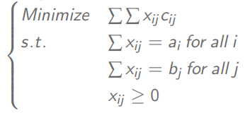
Let a_i the quantity of the commodity available at origin i; bj or the quantity of product required for destination j; vs_ij the cost of transporting a unit of a commodity from origin i to destination j; and x_ij is the quantity transported from origin i to destination j.

Here is the problem :

If the sum of the sources is equal to the sum of the demands, the problem is said to be balanced, in which case the constraints become equalities. Otherwise, a virtual demand point (dummy) is created corresponding to the excess supply and with zero transport cost.

The transport problem is often represented as a bipartite graph with a flow (coupling) problem. Here we will show other variants to solve this problem.