Contents

Constraint programming

The constraint programming solves decision-making problems. An optimization problem is solved successively after several decision problems. For example to determine a shortest way, we will seek to find a path of less than 100 (possible), then less than 50 (impossible), then less than 75, etc. until the optimal solution is found. PPC has a broader field of action than exact methods or metaheuristics.

Definition

PPC solves a constraint satisfaction problem (CSP).

The latter is defined by a triplet with X the set of variables, D the set of domains and C the set of constraints. Domaine D_i is the set of possible values for the variable X_i. Each constraints C_j is defined by its arity (the number of variables on which it relates), the list of these variables and the set of tuples which satisfy it.

Let's take an example of a triplet:

variables: A, B, C, D
areas :
- D_TO = {1,4,5,8}
- D_B = {2,3,5,7,9}
- D_VS = {4,8,9}
- D_D = {1,4,5,7,9}
constraints:
- VS₁(A, C): {(1.7); (1.9); (5.9); (8.9)}
- VS₂(A, D): (1.1); (1.5); (5.5); (5.9); (8.9)}
- VS₃(C, D): {(4.1); (8.1); (9.7)}
- VS₄(B, D): {(2.7); (2.9); (5.8); (7.9); (9.9)}

It is possible to code the constraints in extension, by a set of tuples, or in intention, using operators whose semantics are known. An instantiation is a complete assignment of values to variables, for example { , , , }. Instantiation is a valid solution if the values given to the variables of which such as all the constraints are verified.

We speak of partial or total instantiation (whether it takes all the variables or not), and inconsistent or consistent (whether it validates the constraints or not). A valid solution is therefore a total and consistent instantiation.

Naive resolution: Generate & Test

We generate all the possible assignments. Then we check if they are consistent, as soon as an assignment is consistent we have a valid solution.

If we have a problem with n variables, each can only take two values, the processor does 1,000,000,000 calculations per second. For 30 variables, the resolution take at most 1s, for 50 variables, we go to 11 days; for 70 variables it is necessary to wait 317 centuries.

Backtrack resolution

We generate the assignment tree and then in-depth journey. If a partial assignment (during the traversal) is inconsistent, then the corresponding subtree is cut.

It is akin to Branch & Cut.

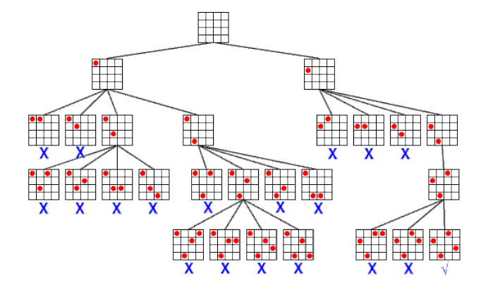
This method does not generate the entire possibility tree unlike the naive method. On the other hand all the constraints are tested with each partial assignment and the convergence time also depends on the order of the variables.

Resolution by stress propagation

This method consists in propagating the constraints in the domain of the variables.

For example let us take x between 0 and 10 and y between 3 and 9; then with the constraint x> y we can restrict the domain of X between 4 and 10.

There are three cases where information is propagated:

when a domain is reduced
when one of the domain terminals is changed
when a domain is a singleton.

It is then possible to propagate the information once (node-consistency), twice (arc-consistency) or more.

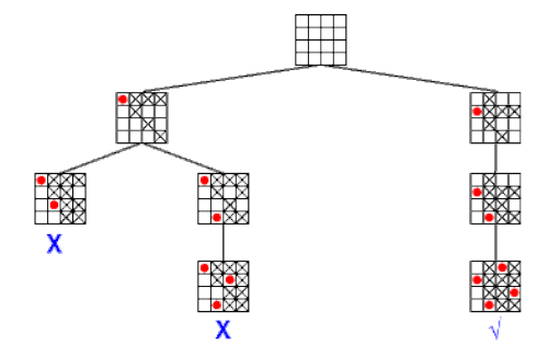
In the node-consistency, for each variable X_i unaffected in A, we subtract from D_Xi any value v such that the assignment A ∪ {(X_i, v)} is inconsistent. The authorized values are propagated in depth.

In the arc-consistency, for each variable X_i unaffected in A, we subtract from D_Xi any value v such that there is a variable X_j unassigned for which, for any value w of D_Xj, the assignment A ∪ {(X_i, v); (X_j, w)} is inconsistent. The authorized values are propagated in depth.

The larger the comparison tuple, the greater the computation time to define the valid domain of the variables. Arc-consistency is less efficient than knot-consistency if the domains are large.