Backpropagation

Backpropagation

Feedforward neural networks are inspired by the processing of information from one or more neuron cells (called neurons). A neuron accepts input signals through its axon, which transmits the electrical signal to the cell body. Dendrites transmit the signal to synapses, which are the connections of the dendrites of one cell to the axons of other cells.

In a synapse, electrical activity is converted into molecular activity (molecules of neurotransmitters crossing the synaptic cleft and binding to receptors). Molecular bonding develops an electrical signal which is transmitted to the axon of connected cells. The backpropagation algorithm is a training regimen for multilayered neural networks with direct action and is not directly inspired by the learning processes of the biological system.

The information processing objective of the technique is to model a given function by modifying the internal weights of the input signals to produce an expected output signal. The system is trained using a supervised learning method, where the error between the system output and a known expected output is presented to the system and used to change its internal state. The state is maintained in a set of weights on the input signals.

The weights are used to represent an abstraction of the mapping of the input vectors to the output signal for the examples to which the system was exposed during training. Each layer of the network provides an abstraction of the information processing of the previous layer, allowing the combination of sub-functions and higher order modeling.

The backpropagation algorithm is a method of learning weights in a multilayer feedback neural network. As such, it requires the definition of a network structure of one or more layers where one layer is fully connected to the next layer. A standard network structure is an input layer, a hidden layer, and an output layer. The method mainly concerns the adaptation of the weights to the calculated error in the presence of input patterns, and the method is applied behind the output layer of the network to the input layer.

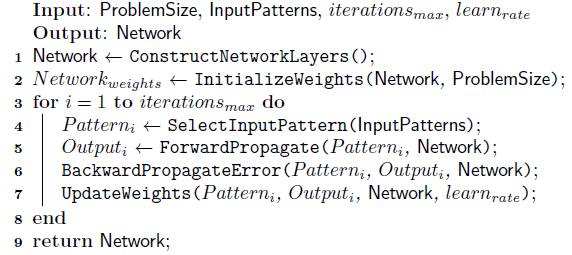
The following algorithm provides a pseudocode to prepare a network using the backpropagation method. A weight is initialized for each input plus an additional weight for a constant bias input which is almost always set to 1.0. The activation of a single neuron on a given input pattern is calculated as follows:

where n is the number of weights and entries, x_ki is the k-th attribute on the i-th entry pattern, and w_bias is the bias weight. A logistic (sigmoid) transfer function is used to calculate the output of a neuron in [0; 1] and provides non-linearities between the input and output signals: 1 / (1 + exp (-a)), where a represents the activation of neurons.

The weighting updates use the delta rule, in particular a modified delta rule in which the error is propagated backward through the network, starting at the output layer and weighted through the previous layers. The following describes the reverse propagation of error and weight updates for a single model.

An error signal is calculated for each node and sent back through the network. For output nodes, this is the sum of the error between node outputs and expected outputs:

where es_i is the error signal for the i-th node, c_i is the expected output and o_i is the actual output for the i-th node. The term td is the derivative of the output of the i-th node. If the sigmod transfer function is used, td_i would be o_i * (1-o_i). For hidden nodes, the error signal is the sum of the weighted error signals of the next layer.

where es_i is the error signal for the i-th node, w_ik is the weight between the i-th and the k-th nodes, and es_k is the error signal for the k-th node.

The error derivatives for each weight are calculated by combining the input from each node and the error signal for the node.

where ed_i is the error derivative for the i-th node, es_i is the error signal for the i-th node and x_k is the input of the k-th node in the previous layer. This process includes the bias which has a constant value.

The weights are updated in a direction that reduces the error derivative ed_i (error assigned to the weight), measured by a learning coefficient.

where w_i (t + 1) is the i-th updated weight, ed_k is the error derivative for the k-th node, and learn_rate is an update coefficient parameter.

The backpropagation algorithm can be used to train a multilayer network to approximate arbitrary nonlinear functions and can be used for problems of regression or classification.

The input and output values must be normalized such that x is in [0; 1]. Initial weights are usually small random values in [0; 0.5]. Weights can be updated either online (after exposure to each input pattern) or in batches (after a fixed number of patterns have been observed). Batch updates should be more stable than online updates for some complex issues.

A logistic (sigmoid) transfer function is commonly used to transfer activation to a binary output value, although other transfer functions can be used such as hyperbolic tangent (tanh), Gaussian, and softmax. It is recommended that you expose the system to input patterns in a different random order on each iteration.

Typically a small number of layers are used, 2 to 4, since increasing the number of layers leads to an increase in the complexity of the system and the time required to train the weights. The rate of learning can vary during training, and it is common to introduce a momentum term to limit the rate of change. The weights of a given network can be initialized with a global optimization method before being refined using the backpropagation algorithm.

One exit node is common for regression problems, just as one exit node per class is common for classification problems.