Contents
ToggleTime Series Forecasting with AutoGluon
Introduction to Amazon AutoGluon's Multimodal AutoML library with a time series forecasting problem.

Introduction to AutoGluon
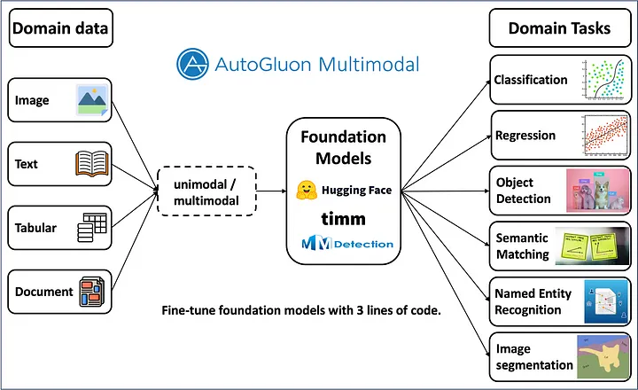
AutoGluon is an open source multimodal python library for AutoML, launched by Amazon. Built on PyTorch, the library uses state-of-the-art models (SOTA) to obtain the best performing models for various machine learning problems.
Equipped with SOTA Deep Learning models, AutoGluon offers solutions to problems such as image classification, object detection, text prediction, image segmentation, time series forecasting and much more, such as in the cover image. This page aims to show readers how to use AutoGluon for a time series forecasting task considering the famous Airlines dataset with minimal code.
It is advisable to create a new Python environment for Autogluon experiments to avoid conflicts with other libraries. Once the new environment is created, install Autogluon by running the command below.
pip install autogluon
import autogluon
AutoGluon TimeSeriesPredictor expects data in a specific format with multi-indexes. One index should be the timestamp and the other should be a unique identifier (it can be any value). A normal pandas data frame can be converted to this format using TimeSeriesDataFrame.from_data_frame().
from autogluon.timeseries import TimeSeriesPredictor, TimeSeriesDataFrame
Let's start by loading the data and placing it in a Time Series DataFrame:
import panda ace pd
data = pd.read_excel('airlinesData.xlsx')
data['Month'] = pd.to_datetime(data['Month']) #convert to datetime
id = ['airline'] * then(data) #create list of id to add to dataframe
data['id'] = id #add new column 'id' to dataframe
data = TimeSeriesDataFrame.from_data_frame(
data,
id_column=”id”,
timestamp_column=”Month”
)
data.tail()
Then we split the data (be careful here we did not do cross-validation):
data.shape
(96, 3)
data.columns
Index(['Passengers'], dtype='object')
»'split data into train and test''
train = data.head(77)
test = data.tail(19)
How to train the preacher
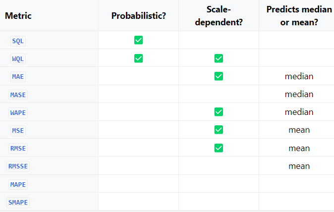
The evaluation metric you choose depends on whether you need a probabilistic forecast or a point forecast. A table containing different measurements is shown below.
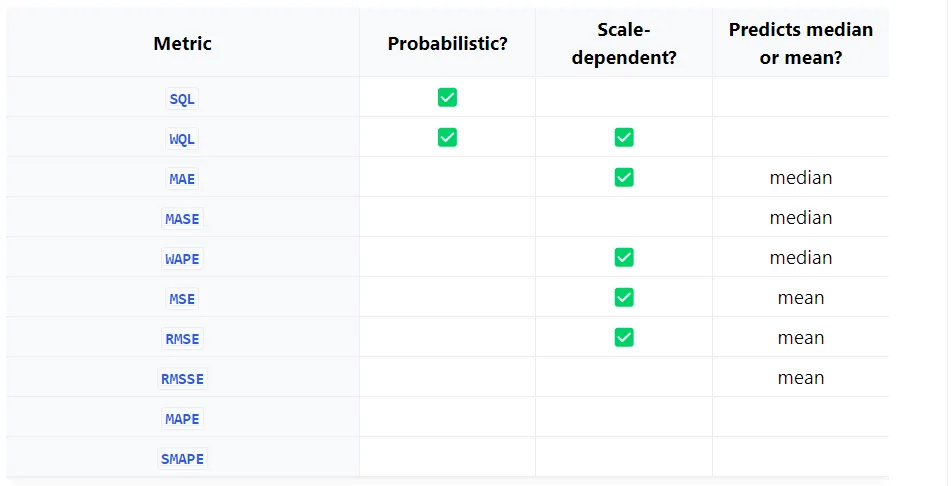
Different models trained on the train data, chosen parameters and evaluation metric can be viewed in the training log. The library leverages statistical models and SOTA Deep Learning models for training. By default, a WeightedEnsemble model will also be tried by the model. it can be disabled by setting activate_ensemble = False in the .fit() method.
predictor = TimeSeriesPredictor(target='Passengers',
                                prediction_length=19,
                                 eval_metric="MASE",).fit(train)
No path specified. Models will be saved in: "AutogluonModels\ag-20240202_034220"
Beginning AutoGluon training...
AutoGluon will save models to 'AutogluonModels\ag-20240202_034220'
=================== System Info ===================
AutoGluon Version: 1.0.0
Python Version: 3.8.18
Operating System: Windows
Platform Machine: AMD64
Platform Version: 10.0.22621
CPU Count: 12
GPU Count: 0
Memory Avail: 0.59 GB / 7.33 GB (8.0%)
Disk Space Avail: 262.60 GB / 476.08 GB (55.2%)
===================================================
Fitting with arguments:
{'enable_ensemble': True,
'eval_metric': MASE,
'hyperparameters': 'default',
'known_covariates_names': [],
'num_val_windows': 1,
'prediction_length': 19,
'quantile_levels': [0.1, 0.2, 0.3, 0.4, 0.5, 0.6, 0.7, 0.8, 0.9],
'random_seed': 123,
'refit_every_n_windows': 1,
'refit_full': False,
'target': 'Passengers',
'verbosity': 2}
Inferred time series frequency: 'MS'
Provided train_data has 77 rows, 1 time series. Median time series length is 77 (min=77, max=77).
Provided dataset contains following columns:
target: 'Passengers'
AutoGluon will gauge predictive performance using evaluation metric: 'MASE'
This metric's sign has been flipped to adhere to being higher_is_better. The metric score can be multiplied by -1 to get the metric value.
===================================================
Starting training. Start time is 2024-02-02 09:12:20
Models that will be trained: ['SeasonalNaive', 'CrostonSBA', 'NPTS', 'AutoETS', 'DynamicOptimizedTheta', 'AutoARIMA', 'RecursiveTabular', 'DirectTabular', 'DeepAR', 'TemporalFusionTransformer', 'PatchTST' ]
Training timeseries model SeasonalNaive.
-0.8728 = Validation score (-MASE)
0.02 s = Training runtime
6.75 s = Validation (prediction) runtime
Training timeseries model CrostonSBA.
-1.4745 = Validation score (-MASE)
0.00 s = Training runtime
15.24 s = Validation (prediction) runtime
Training timeseries model NPTS.
-2.3546 = Validation score (-MASE)
0.02 s = Training runtime
2.85 s = Validation (prediction) runtime
Training timeseries model AutoETS.
-0.8152 = Validation score (-MASE)
0.02 s = Training runtime
30.67 s = Validation (prediction) runtime
Training timeseries model DynamicOptimizedTheta.
-1.4460 = Validation score (-MASE)
0.02 s = Training runtime
29.97 s = Validation (prediction) runtime
Training timeseries model AutoARIMA.
-0.7476 = Validation score (-MASE)
0.02 s = Training runtime
21.59 s = Validation (prediction) runtime
Training timeseries model RecursiveTabular.
-0.5560 = Validation score (-MASE)
4.89 s = Training runtime
0.38 s = Validation (prediction) runtime
Training timeseries models DirectTabular.
-3.5581 = Validation score (-MASE)
0.65 s = Training runtime
0.08 s = Validation (prediction) runtime
Training timeseries models DeepAR.
-1.1489 = Validation score (-MASE)
55.81 s = Training runtime
0.08 s = Validation (prediction) runtime
Training timeseries model TemporalFusionTransformer.
-0.8554 = Validation score (-MASE)
144.14 s = Training runtime
0.02 s = Validation (prediction) runtime
Training timeseries model PatchTST.
-0.9520 = Validation score (-MASE)
32.19 s = Training runtime
0.03 s = Validation (prediction) runtime
Fitting simple weighted together.
Ensemble weights: {'AutoARIMA': 0.09, 'NPTS': 0.07, 'RecursiveTabular': 0.04, 'SeasonalNaive': 0.35, 'TemporalFusionTransformer': 0.44}
-0.2127 = Validation score (-MASE)
1.67 s = Training runtime
31.59 s = Validation (prediction) runtime
Complete training. Models trained: ['SeasonalNaive', 'CrostonSBA', 'NPTS', 'AutoETS', 'DynamicOptimizedTheta', 'AutoARIMA', 'RecursiveTabular', 'DirectTabular', 'DeepAR', 'TemporalFusionTransformer', 'PatchTST', 'WeightedEnsemble ']
Total runtime: 347.54 s
Best model: WeightedEnsemble
Best model score: -0.2127See the results
To do this, simply use the function:
predictor.leaderboard()
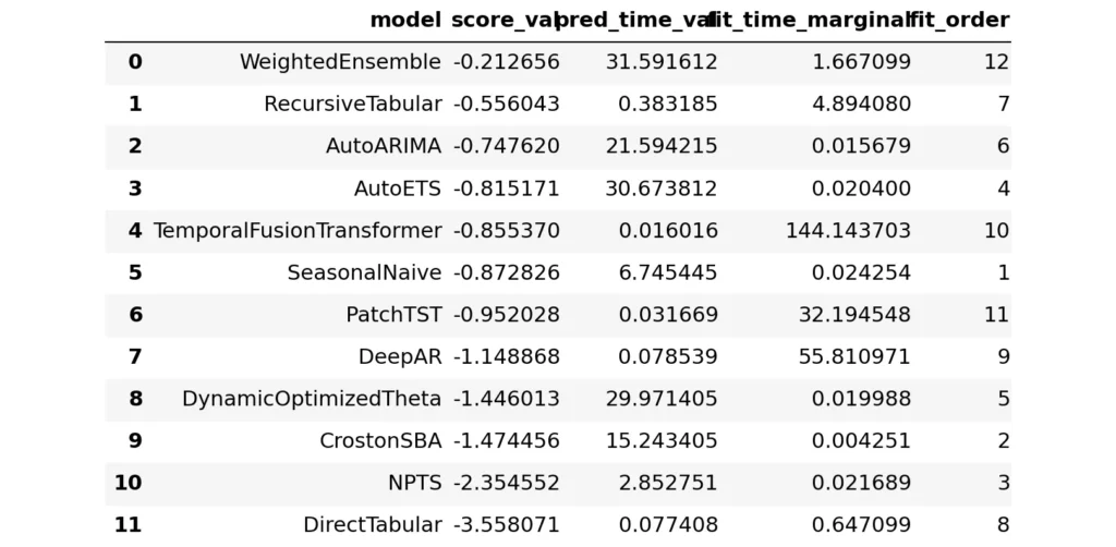
Without specifying a model, the predictor will consider the best prediction model which is WeightedEnsemble in this case.
predictions = predictor.predict(train) predictions Model not specified in prediction, will default to the model with the best validation score: WeightedEnsemble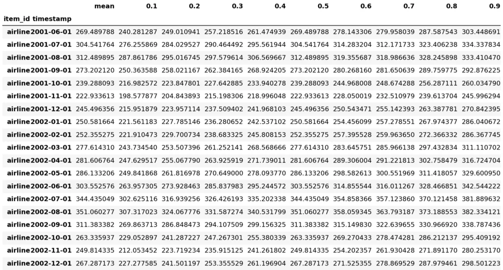
By default, AutoGluon predicts quantile levels [0.1, 0.2, 0.3, 0.4, 0.5, 0.6, 0.7, 0.8, 0.9]. To predict a different set of quantiles, you can use the quantile_levels arguments like:
predictor = TimeSeriesPredictor(eval_metric=”WQL”,quantile_levels=[0.1, 0.5, 0.75, 0.9]) [2].
It is also possible to display the prediction:
import matplotlib.pyplot as plt plt.figure(figsize=(20, 3)) item_id = "airline" y_past = train.loc[item_id]["Passengers"] y_pred = predictions.loc[item_id] y_test = test.loc[ item_id]["Passengers"] plt.plot(y_past, label="Past time series values") plt.plot(y_pred["mean"], label="Mean forecast") plt.plot(y_test, label="Future time series values") plt.fill_between( y_pred.index, y_pred["0.1"], y_pred["0.9"], color="red", alpha=0.1, label=f"10%-90% confidence interval" ) plt. legend();
To use a specific model from the trained models, choose from the ranking or the available models can be seen with the following piece of code.
Using DeepAR
A preferred model can be chosen in Model Zoo and used. By choosing DeepAR as the model of interest, training can be performed as below.
predictor = TimeSeriesPredictor(target='Passengers', prediction_length=19).fit(
   train,
   hyperparameters={
      "DeepAR": {},
   },
)
Beginning AutoGluon training...
AutoGluon will save models to 'AutogluonModels\ag-20240201_193851'
=================== System Info ===================
AutoGluon Version: 1.0.0
Python Version: 3.8.18
Operating System: Windows
Platform Machine: AMD64
Platform Version: 10.0.22621
CPU Count: 12
GPU Count: 0
Memory Avail: 1.51 GB / 7.33 GB (20.6%)
Disk Space Avail: 262.48 GB / 476.08 GB (55.1%)
===================================================Fitting with arguments:
{'enable_ensemble': True,
'eval_metric': WQL,
'hyperparameters': {'DeepAR': {}},
'known_covariates_names': [],
'num_val_windows': 1,
'prediction_length': 19,
'quantile_levels': [0.1, 0.2, 0.3, 0.4, 0.5, 0.6, 0.7, 0.8, 0.9],
'random_seed': 123,
'refit_every_n_windows': 1,
'refit_full': False,
'target': 'Passengers',
'verbosity': 2}
Inferred time series frequency: 'MS'
Provided train_data has 77 rows, 1 time series. Median time series length is 77 (min=77, max=77).
Provided dataset contains following columns:
target: 'Passengers'
AutoGluon will gauge predictive performance using evaluation metric: 'WQL'
This metric's sign has been flipped to adhere to being higher_is_better. The metric score can be multiplied by -1 to get the metric value.
===================================================
Starting training. Start time is 2024-02-02 01:08:51
Models that will be trained: ['DeepAR']
Training timeseries models DeepAR.
-0.1003 = Validation score (-WQL)
50.19 s = Training runtime
0.11 s = Validation (prediction) runtime
Not fitting ensemble as only 1 model was trained.
Complete training. Models trained: ['DeepAR']
Total runtime: 50.33 s
Best model: DeepAR
Best model score: -0.1003
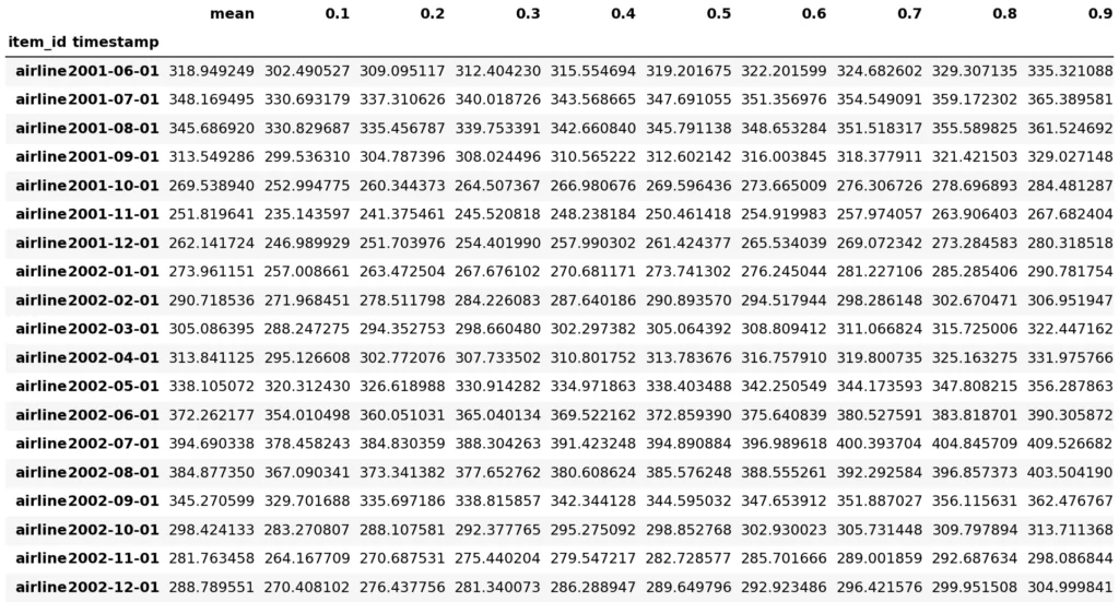
predictions = predictor1.predict(train)
predictions
Model not specified in prediction, will default to the model with the best validation scorepredictions = predictor.predict(train)
predictions
import matplotlib.pyplot as plt
plt.figure(figsize=(20, 3))
item_id = “airline”
y_past = train.loc[item_id][“Passengers”]
y_pred = predictions.loc[item_id]
y_test = test.loc[item_id][“Passengers”]
plt.plot(y_past, label=”Past time series values”)
plt.plot(y_pred[“mean”], label=”Mean forecast”)
plt.plot(y_test, label=”Future time series values”)
plt.fill_between(
y_pred.index, y_pred[“0.1”], y_pred[“0.9″], color=”red”, alpha=0.1, label=f”10%-90% confidence interval”
)
plt.legend();

The models auto-tune to find the best setting. AutoGluon is an autoML tool, the user does not need to tune the models themselves.
List of methods
Naive model – Reference model that sets the forecast equal to the last observed value.
SeasonalNaiveModel – Reference model that sets the forecast equal to the last observed value for the same season.
Average model – Reference model that sets the forecast equal to the historical mean or quantile.
SeasonalAverageModel – Reference model that sets the forecast equal to the historical average or quantile of the same season.
Model Zero – A naive forecaster who always returns 0 forecasts over the forecast horizon, where forecast intervals are calculated using a conforming prediction.
ETS Model – Exponential smoothing with trend and seasonality.
AutoARIMA Model – ARIMA model set automatically.
AutoETS Model – Automatically adjusted exponential smoothing with trend and seasonality.
AutoCES Model – Forecasting with a complex exponential smoothing model where model selection is performed using the Akaike Information Criterion.
ThetaModel – Theta prediction model [Assimakopoulos2000].
ADIDAModel – Intermittent demand forecasting model using the global-disaggregated intermittent demand approach [Nikolopoulos2011].
CrostonClassicModel – Intermittent demand forecasting model using the Croston model where the smoothing parameter is set to 0.1 [Croston1972].
CrostonOptimized model – Intermittent demand forecasting model using the Croston model where the smoothing parameter is optimized [Croston1972].
CrostonSBAModel – Intermittent demand forecasting model using the Croston model with the Syntetos-Boylan bias correction approach [SyntetosBoylan2001].
IMAPA Model – Intermittent Demand Forecasting Model Using Intermittent Multiple Aggregation Forecasting Algorithm [Petropoulos2015].
NPTS Model – Nonparametric Time Series Forecaster.
DeepAR Model – Autoregressive forecasting model based on recurrent neural network [Salinas2020].
DLinearModel – Simple feedback neural network that subtracts trend before forecasting [Zeng2023].
PatchTSTModel – Transformer-based forecaster that segments each time series into patches [Nie2023].
SimpleFeedForwardModel – Simple feedback neural network that simultaneously predicts all future values.
Temporal Fusion Transformer Model – Combines LSTM with a transformer layer to predict quantiles of all future target values [Lim2021].
WaveNet Model – WaveNet estimator that uses the architecture proposed in [Oord2016] with quantized targets.
Direct TabularModel – Simultaneously predict all future time series values using AutoGluon-Tabular's TabularPredictor.
Recursive TabularModel – Predict future time series values one by one using AutoGluon-Tabular's TabularPredictor.
Choice of metrics
Choosing the right evaluation metric is one of the most important choices when using an AutoML framework. This page lists the forecast evaluation metrics available in AutoGluon, explains when different metrics should be used, and describes how to define custom evaluation metrics.
When using AutoGluon, you can specify the metric using the eval_metric argument of TimeSeriesPredictor, for example:
from autogluon.timeseries import TimeSeriesPredictor
predictor = TimeSeriesPredictor(eval_metric=”MASE”)
AutoGluon always reports all measurements in a “higher is better” format. For this purpose, certain metrics are multiplied by -1. For example, if we set eval_metric=”MASE”, the predictor will actually report -MASE (i.e. MASE score multiplied by -1). This means that the test_score will be between 0 (most accurate prediction) and (least accurate prediction).
Currently, AutoGluon supports the following evaluation metrics:
SQL Scaled quantile loss.
WQL Weighted quantile loss.
MAE Mean absolute error.
MAPE Mean absolute error in percentage.
MASE Mean absolute scale error.
MSE Mean squared error.
RMSE Mean square error.
RMSSE Mean squared scale error.
SMAPE Symmetric mean absolute percentage error.
WAPE Weighted absolute percentage error.
You can also define a custom forecast evaluation metric.
If you're unsure which evaluation metric to choose, here are three questions that can help you make the right choice for your use case.
1. Are you interested in a point forecast or a probabilistic forecast?
If your goal is to generate an accurate probabilistic forecast, you should use WQL or SQL metrics. These metrics are based on quantile loss and measure the accuracy of quantile predictions. By default, AutoGluon predicts quantile levels [0.1, 0.2, 0.3, 0.4, 0.5, 0.6, 0.7, 0.8, 0.9]. To predict a different set of quantiles, you can use the quantile_levels argument:
predictor = TimeSeriesPredictor(eval_metric= »WQL », quantile_levels=[0.1, 0.5, 0.75, 0.9])
All other forecast measures described on this page are point forecast measures. Note that if you select eval_metric for a point forecast metric when creating the TimeSeriesPredictor, the forecast minimizing that metric will always be provided in the "average" column of the predictions data frame.
2. Do you care more about accurately predicting time series with large values?
If the answer is "yes" (for example, if it is important to more accurately predict sales of popular products), you should use scale-dependent metrics such as WQL, MAE, RMSE, or WAPE. These metrics are also well suited to processing sparse (intermittent) time series with many zeros.
If the answer is "no" (you care equally about all time series in the dataset), consider scaled metrics such as SQL, MASE, and RMSSE. Alternatively, the percentage-based measures MAPE and SMAPE can also be used to equalize the scale between time series. However, these percentage-based measures have some well-documented limitations, so we do not recommend using them in practice. Note that scaled and percentage-based metrics are poorly suited to sparse (intermittent) data.
3. (Point forecast only) Do you want to estimate the mean or the median?
To estimate the median, you should use metrics like MAE, MASE, or WAPE. If your goal is to predict the mean (expected value), you should use the MSE, RMSE, or RMSSE metrics.
