Contents
TogglePipeline Forecasting with method comparison
In this tutorial, you will learn pipeline forecasting: how to compare and select time series models based on performance

Preview
In the first part, you will learn about many time series models. This part is divided into three parts:
- classic time series models,
- supervised models,
- and models based on deep learning.
In the second part, you will see an application to a use case in which you will build some time series models for stock market forecasting and you will learn some time series modeling techniques. The models will be compared to each other to select the best performing one.
Preprocessing
Due to the nature of time series data, time series modeling has a number of specifics that are not relevant to other data sets.
The first specificity of time series is that the timestamp that identifies the data has intrinsic meaning. Univariate time series models are forecasting models that use a single variable (the target variable) and its temporal variation to predict the future. Univariate models are specific to time series.
In other situations, you may have additional explanatory data about the future. For example, imagine you want to factor weather forecasts into your product demand forecasts, or you have other data that will influence your forecasts. In this case, you can use multivariate time series models.
Multivariate time series models are univariate time series models adapted to incorporate external variables. You can also use supervised machine learning for this task.
If you want to use temporal variation on your time series data, you will first need to understand the different types of temporal variation you can expect.
Time series decomposition is a technique for extracting multiple types of variation from your data set. There are three important components in time series temporal data: seasonality, trend, and noise.
Seasonality is a recurring movement present in your time series variable. For example, the temperature of a location will be higher during the summer months and lower during the winter months. You can calculate average monthly temperatures and use this seasonality as a basis for predicting future values.
A trend can be a long-term upward or downward trend. In a time series of temperatures, a trend could be present due to global warming. For example, in addition to summer/winter seasonality, you might see a slight increase in average temperatures over time.
Noise is part of the variability of a time series that cannot be explained by seasonality or a trend. When creating models, you end up combining different components into a mathematical formula. Two elements of such a formula can be seasonality and trend. A model that combines the two will never perfectly represent temperature values: an error will always remain. This is represented by the noise figure.
Let's see a short example to understand how to decompose a time series in Python, using the CO2 dataset from the statsmodels library.
You can import the data as follows:
import statsmodels.datasets.co2 as co2
co2_data = co2.load().data
print(co2_data)
There are a few NA values that you can remove using interpolation, as follows:
co2_data = co2_data.fillna(co2_data.interpolate())
You can see the temporal evolution of the CO2 values using the following code:
co2_data.plot()
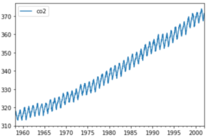
You can perform out-of-the-box decomposition using the statsmodels season_decompose function. The following code will generate a plot that divides the time series into trend, seasonality, and noise (here called residual):
from statsmodels.tsa.seasonal import seasonal_decompose
result = seasonal_decompose(co2_data)
result.plot()
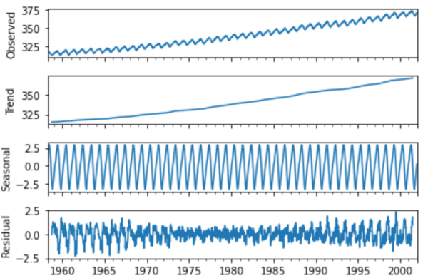
The breakdown of CO2 data shows an upward trend and strong seasonality.
Correlation search
Let's move on to the second type of temporal information that can be present in time series data: autocorrelation.
The autocorrelation is the correlation between the current value of a time series and past values. If so, you can use current values to better predict future values.
Autocorrelation can be positive or negative:
- Positive autocorrelation means that a high value now is likely to produce a high value in the future and vice versa. Think about the stock market: if everyone buys a stock, then the price increases. When the price goes up, people think it's a good stock to buy and they buy it too, which pushes the price up further. However, if the price falls, then everyone fears a crash, sells their shares and the price falls.
- Negative autocorrelation is the opposite: a high value today implies a low value tomorrow, and a low value today implies a high value tomorrow. A common example is rabbit populations in natural environments. If there are a lot of wild rabbits over the course of a summer, they will eat all available natural resources. During the winter there will be nothing left to eat, so many of them will die and the population of surviving rabbits will be small. During this year with a small rabbit population, natural resources will grow and allow the rabbit population to grow the following year.
Two famous graphs can help you detect autocorrelation in your data set: the ACF plot and the PACF plot.
You can calculate an ACF plot using Python as follows:
from statsmodels.graphics.tsaplots import plot_acf
plot_acf(co2_data)

On the x-axis you can see the time steps (back in time). This is also called the number of shifts. On the y-axis you can see how closely each time step correlates with “present” time. It is evident that there is significant autocorrelation in this graph.
The PACF is an alternative to the ACF. Rather than giving the autocorrelations, it gives you the partial autocorrelation. This autocorrelation is called partial, because at each step back, only one additional autocorrelation is listed. This is different from ACF, because ACF contains duplicate correlations when variability can be explained by multiple points in time.
For example, if today's value is the same as yesterday's value, but also the same as the day before yesterday, the ACF will show two highly correlated steps. The PACF would only display yesterday and delete the day before yesterday.
You can calculate a PACF plot using Python as follows:
from statsmodels.graphics.tsaplots import plot_pacf
plot_pacf(co2_data)
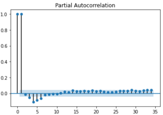
You can see below that this PACF plot gives a much better representation of the autocorrelation in the CO2 data. There is a strong positive autocorrelation with lag 1: a high value now means you will most likely see a high value in the next step. Since the autocorrelation shown here is partial, you see no duplicate effects with prior lags, making the PACF plot sharper and clearer.
Stationarity
Another important definition of time series is stationarity. A stationary time series is a time series without a trend. Some time series models are not capable of handling trends (more on this later). You can detect non-stationarity using the Dickey-Fuller test and remove non-stationarity using differencing.
The Dickey-Fuller test is a statistical hypothesis test that can detect non-stationarity. You can use the following Python code to apply a Dickey-Fuller test to CO2 data:
from statsmodels.tsa.stattools import adfuller
adf, pval, usedlag, nobs, crit_vals, icbest = adfuller(co2_data.co2.values)
print('ADF test statistic:', adf)
print('ADF p-values:', pval)
print('ADF number of lags used:', usedlag)
print('ADF number of observations:', nobs)
print('ADF critical values:', crit_vals)
print('ADF best information criterion:', icbest)

The null hypothesis of the ADF test is that a unit root is present in the time series. The alternative hypothesis is that the data are stationary.
The second value is the p-value. If this p-value is less than 0.05, you can reject the null hypothesis (reject non-stationarity) and accept the alternative hypothesis (stationarity). In this case, we cannot reject the null hypothesis and it will be necessary to assume that the data are non-stationary. As you have seen the data, you know that there is a trend, so this also confirms the result that we got.
Differentiation
You can remove the trend from your time series. The goal is to only have seasonal variations: this can be a way to use certain models that work with seasonality but not with trends.
prev_co2_value = co2_data.co2.shift()
differenced_co2 = co2_data.co2 – prev_co2_value
differenced_co2.plot()
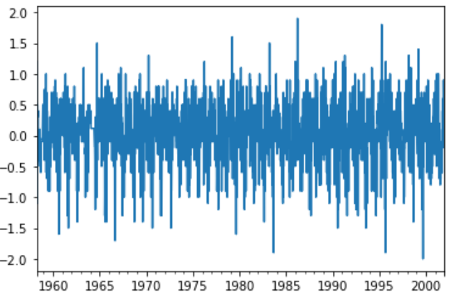
If you repeat the ADF test on the differentiated data, you will confirm that this data is now indeed stationary:
adf, pval, usedlag, nobs, crit_vals, icbest = adfuller(differenced_co2.dropna())
print('ADF test statistic:', adf)
print('ADF p-values:', pval)
print('ADF number of lags used:', usedlag)
print('ADF number of observations:', nobs)
print('ADF critical values:', crit_vals)
print('ADF best information criterion:', icbest)

The p-value is very low, indicating that the alternative hypothesis (stationarity) is true.
Smoothing in case of significant noise
Exponential smoothing is a basic statistical technique that can be used to smooth time series. Time series models often have high long-term variability, but also (noisy) short-term variability. Smoothing allows you to make your curve smoother so that long-term variability becomes more evident and short-term (noisy) patterns are removed.
This smoothed version of the time series can then be used for analysis.
If you want to go even further, you can use triple exponential smoothing, also called Holt Winter exponential smoothing. You should only use it when there are three important signals in your time series data. For example, one signal could be the trend, another could be weekly seasonality, and a third could be monthly seasonality.
In the following example, you see how to apply simple exponential smoothing to CO2 data. The smoothness level indicates how smooth your curve should become. In the example it is set very low, indicating a very gentle curve. Feel free to play around with this setting and see what less smooth versions look like.
from statsmodels.tsa.api import SimpleExpSmoothing
es = SimpleExpSmoothing(co2_data.co2.values)
es.fit(smoothing_level=0.01)
plt.plot(co2_data.co2.values)
plt.plot(es.predict(es.params, start=0, end=None))
plt.show()
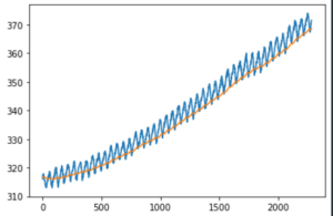
Once the curve is smoothed, it is much easier to learn (here it amounts to doing the trend).
One-step or multi-step models (oneshot or autoregressive)
The final concept that is important to understand before getting started with modeling is single-stage versus multi-stage models.
Some models work very well at predicting the next step in a time series, but lack the ability to predict multiple steps at once. These models are one-step models. You can build multi-step models with them by windowing your predictions, but there is a risk: when you use predicted values to make predictions, your errors can quickly accumulate and become very large.
Multi-stage models are models that have the intrinsic ability to predict several stages at once. They are generally the best choice for long-term forecasts, and sometimes also for single-step forecasts. It is essential that you decide how many steps you want to predict before you start creating models. It just depends on your use case.
Model Types
Now that you've seen the main specifics of time series data, it's time to look at the types of models that can be used to predict time series. This task is usually called forecasting.
Classic time series models
Classic time series models are a family of models traditionally widely used in many areas of forecasting. They are heavily based on temporal variation within a time series and work well with univariate time series. Some advanced options exist to also add external variables into models. These models generally only apply to time series and are not useful for other types of machine learning.
Supervised models
Supervised models are a family of models used for many machine learning tasks. A machine learning model is supervised when it uses clearly defined input variables and one or more output (target) variables.
Supervised models can be used for time series, provided you have a way to extract the seasonality and put it into a variable. Examples include creating a variable for a year, month, or day of the week, etc. These are then used as X variables in your supervised model and the “y” is the actual value of the time series. You can also include lagged versions of y (the past value of y) in the X data, to add autocorrelation effects.
Deep learning and recent models
The growing popularity of deep learning in recent years has also opened new doors for prediction, as specific deep learning architectures have been invented that work very well on sequence data.
Cloud computing and the popularization of AI as a service have also given rise to a number of new inventions in the field. Facebook, Amazon and other big tech companies are opening up their forecasting products or making them available on their cloud platforms. The availability of these new "black box" models gives forecasters new tools to try and test, and can sometimes even outperform previous models.
Classic model (AutoARIMA)
The ARIMA model family is a set of smaller models that can be combined. Each part of the ARIMA model can be used as a stand-alone component, or the different basic elements can be combined. When all the individual components are assembled, you get the SARIMAX model.
The difficulty with ARIMA or SARIMAX models is that you have many parameters (pp, d, q) or even (p, d, q)(P, D, Q) that you have to choose.
In some cases, you can inspect autocorrelation plots and identify logical choices for parameters. You can use the statsmodels implementation of SARIMAX and test performance with parameters of your choice.
Another approach is to use an auto-arima function that automatically optimizes the hyperparameters for you. The Pyramid Python library does just that: it tries different combinations and selects the one with the best performance.
import pmdarima as pm
from pmdarima.model_selection import train_test_split
import numpy as np
import matplotlib.pyplot as plt
train, test = train_test_split(co2_data.co2.values, train_size=2200)
model = pm.auto_arima(train, seasonal=True, m=52)
preds = model.predict(test.shape[0])
plt.plot(co2_data.co2.values[:2200], train)
plt.plot(co2_data.co2.values[2200:], preds)
plt.show()

In this chart, the blue line represents the actual data (training data) and the orange line represents the forecast.
You might see vector autoregression, or VAR, as a multivariate alternative to Arima. Rather than predicting one dependent variable, you predict multiple time series at the same time. This can be particularly useful when there are strong relationships between your different time series. Vector autoregression, like the standard AR model, contains only an autoregressive component.
The VARMA model is the multivariate equivalent of the ARMA model. VARMA is to ARMA what VAR is to AR: it adds a moving average component to the model.
If you want to go further, you can use VARMAX. The X represents external (exogenous) variables. Exogenous variables are variables that can help your model make better predictions, but do not need to be predicted themselves. Implementing VARMAX statsmodels is a good way to start implementing VARMAX models.
More advanced versions such as Seasonal VARMAX (SVARMAX) exist, but they become so complex and specific that it will be difficult to find implementations to do this easily and efficiently. Once patterns become so complex, it becomes difficult to understand what is going on inside the pattern and it is often best to start looking at other familiar patterns.
Linear regression model
The regression Linear is arguably the simplest supervised machine learning model. Linear regression estimates linear relationships: each independent variable has a coefficient that indicates how that variable affects the target variable.
Simple linear regression is a linear regression in which there is only one independent variable. An example of a simple linear regression model in non-series data could be: hot chocolate sales that depend on the outside temperature (degrees Celsius).
In multiple linear regression, rather than using a single independent variable, you use multiple independent variables. You can imagine that the 2D chart turns into a 3D chart, where the third axis represents the Price variable. In this case, you will build a linear model which explains sales using temperature and price. You can add as many variables as needed.
Of course, this is not a time series dataset: no temporal variables are present. So how could you use this technique for time series? The answer is quite simple. Rather than using only temperature and price in this dataset, you can add the variables year, month, day of the week, etc.
If you are building a supervised model on time series, you have the disadvantage of having to do a bit of feature engineering to extract the seasonality in the variables one way or another. The advantage, however, is that adding exogenous variables becomes much easier.
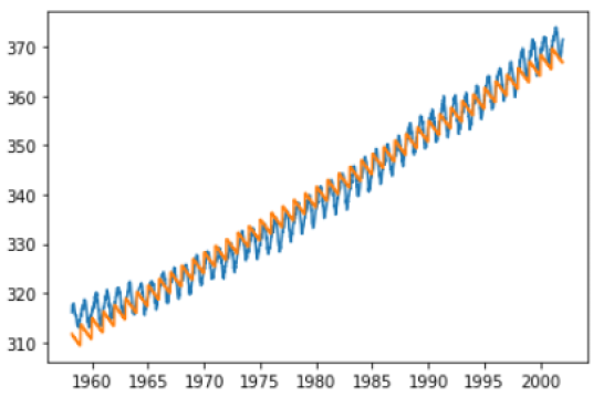
Now let's see how to apply linear regression on the CO2 dataset. You can prepare CO2 data as follows:
import numpy as np
# extract the seasonality data
months = [x.month for x in co2_data.index]
years = [x.year for x in co2_data.index]
day = [x.day for x in co2_data.index]
# convert into one matrix
X = np.array([day, months, years]).T
You then have three independent variables: day, month and week. You can also think about other seasonality variables like day of the week, week number, etc., but for now, let's go with it.
You can then use scikit-learn to create a linear regression model and make predictions to see what the model has learned:
from sklearn.linear_model import LinearRegression
# fit the model
my_lr = LinearRegression()
my_lr.fit(X, co2_data.co2.values)
# forecast on the same period
preds = my_lr.predict(X)
# plot what has been learned
plt.plot(co2_data.index, co2_data.co2.values)
plt.plot(co2_data.index, preds)
Random Forest
The linear model is very limited: it can only fit linear relationships. Sometimes this is enough, but in most cases it is better to use more efficient models. Random Forest is a widely used model for fitting nonlinear relationships. It remains very simple to use.
The scikit-learn library has the RandomForestRegressor which you can simply use to replace the LinearRegression in the previous code.
from sklearn.ensemble import RandomForestRegressor
# fit the model
my_rf = RandomForestRegressor()
my_rf.fit(X, co2_data.co2.values)
# forecast on the same period
preds = my_rf.predict(X)
# plot what has been learned
plt.plot(co2_data.index, co2_data.co2.values)
plt.plot(co2_data.index, preds)

For now, it is enough to understand that this Random Forest was able to learn the training data better. In a later part of this article, you will learn about more quantitative methods for model evaluation.
XGBoost
The XGBoost model is a third model that you absolutely must know. There are many other models, but Random Forests and XGBoost are considered absolute classics among the supervised machine learning family.
XGBoost is a machine learning model based on the gradient enhancement framework. This model is a weak learner ensemble model just like the Random Forest but with an interesting advantage. In standard gradient boosting, individual trees are adjusted in sequence and each tree The consecutive decision tree is adjusted so as to minimize the error of the previous trees. XGBoost achieves the same result but is still able to do learning in parallel.
You can use the XGBoost package as follows:
import xgboost as xgb
# fit the model
my_xgb = xgb.XGBRegressor()
my_xgb.fit(X, co2_data.co2.values)
# forecast on the same period
preds = my_xgb.predict(X)
# plot what has been learned
plt.plot(co2_data.index, co2_data.co2.values)
plt.plot(co2_data.index, preds)
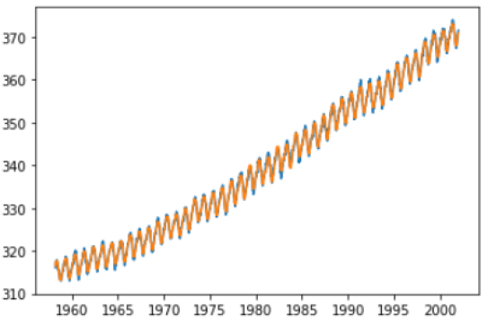
As you can see, this model also fits the data very well. You will learn how to perform model evaluation in the last part of this article.
Other models to implement
GARCH
GARCH stands for Generalized Autoregressive Conditional Heteroskedasticity. This is an approach for estimating the volatility of financial markets and is typically used for this use case. It is rarely used for other use cases.
The model works well for this because it assumes an ARMA model for the error variance of the time series rather than the actual data. This way you can predict variability rather than actual values.
There are a number of variations to the GARCH family of models, for example take a look at this. This model is good to know, but should only be used when forecasting variability is necessary and is therefore relatively different from the other models presented in this article.
TBATS
TBATS represents the combination of the following components:
Trigonometric seasonality
Box-Cox transformation
ARMA errors
Tendency
Seasonal components
The model was created in 2011 as a solution for forecasting time series with multiple seasonal periods. As it is relatively new and relatively advanced, it is less widespread and less used than the models in the ARIMA family.
A useful Python implementation of TBATS can be found in Python's sktime package.
You will now see three newer models that can also be used for forecasting purposes. They are even more complex to understand and master and may (or may not) produce better results, depending on the data and the specifics of the use case.
LSTM (long short-term memory)
LSTMs are networks of neurons recurring. Neural networks are very complex machine learning models that pass input data through a network. Each node in the network learns a very simple operation. The neural network consists of many such nodes. The fact that the model can use a large number of simple nodes makes the overall prediction very complex. Neural networks can therefore adapt to very complex and non-linear data sets.
RNNs are a special type of neural network, in which the network can learn from sequence data. This can be useful for several use cases, notably for understanding time series (which are clearly sequences of values over time), but also text (sentences are sequences of words).
LSTMs are a specific type of RNN. They have repeatedly proven useful for time series forecasting. They require certain data and are more complicated to learn than supervised models. Once you master them, they can be very powerful depending on your data and your specific use case.
To get started with LSTM, the Keras library in Python is an excellent starting point.
Prophet
Prophet is an open source time series library by Facebook. This is a black box model, as it will generate forecasts without much specification from the user. This can be an advantage because you can almost automatically generate forecast models without much knowledge or effort.
On the other hand, there is also a risk: if you don't pay enough attention, you could very well produce a model that looks good for the automated templating tool, but in reality doesn't work. not good.
Thorough model validation and evaluation is recommended when using such black box models, but if you find that they work well in your specific use case, you may find a lot of added value.
You can find many resources on Facebook's GitHub.
DeepAR
DeepAR is another black box model developed by Amazon. The operation is different in depth, but in terms of user experience, it is relatively equal to Prophet. The idea again is to have a Python library that does all the heavy lifting for you.
Again, caution is advised, as a black box model can never be expected to be completely reliable. In the next part, you'll see more about model evaluation and benchmarking, which is extremely important with such complex models. The more complex a model is, the more erroneous it can be!
An interesting and easy-to-use implementation of DeepAR is available in the Gluon package.
How to evaluate models
Time Series Metrics
The first thing to define when selecting models is the metric you want to look at. In the previous part, you saw several fits with different qualities (think linear regression versus random forest).
To take model selection further, you will need to define a metric to evaluate your models. A model very often used in forecasting is the mean square error. This metric measures the error at each moment and takes the square of it. The average of these squared errors is called the mean squared error. An often used alternative is the mean square error: the square root of the mean square error.
Another frequently used measure is the absolute mean error: rather than taking the square of each error, here it takes the absolute value. Mean absolute percentage error is a variation of this where the absolute error at each time point is expressed as a percentage of the true value. This gives a measurement in percentage form, very easy to interpret.
Distribution of training tests in time series
The second thing to consider when evaluating machine learning is to consider that a model that performs well on training data does not necessarily perform well on new out-of-sample data. Such a model is called an overfitting model.
There are two common approaches that can help you estimate whether a model generalizes correctly: split testing and cross-validation.
Train test splitting means that you remove some of your data before fitting the model. As an example, you can remove the last 3 years from the CO2 database and use the remaining 40 years to adjust the model. You would then forecast the three years of test data and measure the evaluation metric of your choice between your predictions and the actual values from the last three years.
To compare and choose models, you can create multiple models on the 40 years of data and perform test set evaluation on each of them. Based on this test performance, you can select the best performing model.
Of course, if you are building a short-term forecasting model, using three years of data would not make sense: you would choose an evaluation period comparable to the period you would actually forecast.
Cross-validation of time series
One risk with train test distribution is that you only measure at one point in time. In non-series data, the test set is usually generated by a random selection of data points. However, in time series this does not work in many cases: when sequences are used, you cannot remove a point from the sequence and still expect the model to work.
Therefore, it is best to apply time series train test distributions by selecting the final period as the test set. The risk here is that it could go wrong if your last period is not very reliable. During the last periods of covid, we can imagine that many economic forecasts have completely deteriorated: the underlying trends have changed.
Cross-validation is a method that performs repeated evaluation of train tests. Rather than splitting a train test, it creates several (the exact number is a user-defined parameter). For example, if you use three-fold cross-validation, you would divide your dataset into three equal parts. You will then fit the same model three times on two-thirds of the dataset and use the other third for evaluation. Ultimately, you have three assessment scores (each on a different set of tests) and you can use the average as your final measure.
By doing this, you avoid randomly selecting a model that works on the test set: you are now assured that it works on multiple test sets.
However, in time series, you cannot apply random selection to obtain multiple test sets. If you did this, you would end up with sequences with many missing data points.
A solution can be found in time series cross-validation. What it does is create multiple train test sets, but each of the test sets corresponds to the end of the period. For example, the first distribution of train tests could be built on the first 10 years of data (5 trains, 5 tests). The second model would be carried out on the first 15 years of data (10 trains, 5 tests), etc. This can work well but has the disadvantage that each of the models does not use the same number of years in the training data.
An alternative is to do a rolling split (always 5 years training, 5 years testing), but the disadvantage here is that you can never use more than 5 years for the training data.
Experiments on time series models
In conclusion, when selecting time series models, it is essential to define the following questions before starting to experiment:
- What metric do you use?
- What period do you want to plan for?
- How do you ensure your model works on future data points that haven't been seen by the model?
Once you have the answer to the above questions, you can start trying different models and use the defined evaluation strategy to select and improve models.
Go further
Concerning the choices mentioned in the previous section, I invite you to read the corresponding tutorials. Good reading !
