Now suppose you have chosen the best possible model for a particular problem and are working to further improve its accuracy. In this case, you will need to apply more advanced machine learning techniques which are collectively referred to as ensemble learning.
A set is a collection of elements that collectively contribute to a whole. A familiar example is a musical ensemble, which mixes the sounds of several musical instruments to create a beautiful harmony, or architectural ensembles, which are a collection of buildings designed as a unit. In ensembles, the (whole) harmonious result is more important than the execution of any individual part.

Contents
TogglePrinciples of ensemble learning
Condorcet's Jury Theorem (1784) is about a set in some sense. It states that, if each member of the jury makes an independent judgment and the probability of each juror's correct decision is greater than 0.5, then the probability of the correct decision of the entire jury increases with the total number of jurors and tends to a. On the other hand, if the probability of being right is less than 0.5 for each juror, then the probability of a correct decision by the jury as a whole decreases with the number of jurors and tends towards zero.
Consider another example of sets: an observation known as Wisdom of the Crowd. In 1906 Francis Galton visited a rural fair in Plymouth where he saw a competition held for farmers. 800 participants tried to estimate the weight of a slaughtered bull. The actual weight of the bull was 1198 pounds. Although none of the farmers could guess the exact weight of the animal, the average of their predictions was 1197 pounds.
A similar idea for error reduction has been adopted in the field of machine learning.
Priming (bagging and bootstrapping)
Bagging (also known as Bootstrap aggregation) is one of the earliest and most basic ensemble techniques. It was proposed by Leo Breiman in 1994. Bagging is based on the bootstrap statistical method, which makes it possible to evaluate many statistics of complex models.
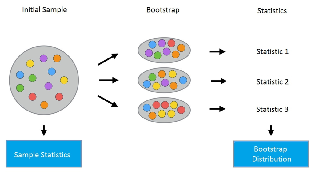
The bootstrap method proceeds as follows. Consider a sample X of size N. A new sample can be made from the original sample by drawing N elements from the latter in a random and uniform manner, with replacement. In other words, we select a random element from the original sample of size N and do it N times. All elements are equally likely to be selected, so each element is drawn with equal probability 1/N.
Let's say we draw balls from a bag one at a time. At each stage, the selected ball is put back in the bag so that the next selection is made in an equiprobable manner, that is to say from the same number of balls N. Note that, since the balls are put back , there may be duplicates in the new sample. Let's call this new sample X1.
By repeating this procedure M times, we create M bootstrap samples X1, …, XM. In the end, we have a sufficient number of samples and can calculate various statistics from the original distribution.
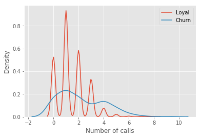
For our example, we'll use the familiar telecom_churn dataset. Previously, when we discussed the importance of features, we saw that one of the most important features in this dataset is the number of customer service calls. Let's visualize the data and look at the distribution of this feature.
| import panda ace pd | |
| from matplotlib import pyplot ace please | |
| please.style.worn('ggplot') | |
| please.rcParams['figure.figsize'] = 10, 6 | |
| import sea born ace sns | |
| %matplotlib inline | |
| telecom_data = pd.read_csv('../../data/telecom_churn.csv') | |
| fig = sns.kdeplot(telecom_data[telecom_data['churn'] == False]['Customer service calls'], | |
| label = 'Loyal') | |
| fig = sns.kdeplot(telecom_data[telecom_data['churn'] == True]['Customer service calls'], | |
| label = 'churn') | |
| fig.set(xlabel='Number of calls', ylabel='Density') | |
| please.show() |
| import numpy ace n.p. | |
| def get_bootstrap_samples(data, n_samples): | |
| “””Generate bootstrap samples using the bootstrap method. » » » | |
| clues = n.p..random.randint(0, then(data), (n_samples, then(data))) | |
| samples = data[clues] | |
| return samples | |
| def stat_intervals(status, alpha): | |
| “””Produce an interval estimate. » » » | |
| boundaries = n.p..percentile(status, [100 * alpha / 2., 100 * (1 – alpha / 2.)]) | |
| return boundaries | |
| # Save the data about the loyal and form customers to split the dataset | |
| loyal_calls = telecom_data[telecom_data['churn'] | |
| == False]['Customer service calls'].values | |
| churn_calls= telecom_data[telecom_data['churn'] | |
| == True]['Customer service calls'].values | |
| # Set the seed for reproducibility of the results | |
| n.p..random.seed(0) | |
| # Generate the samples using bootstrapping and calculate the mean for each of them | |
| loyal_mean_scores = [n.p..mean(sample) | |
| for sample in get_bootstrap_samples(loyal_calls, 1000)] | |
| churn_mean_scores = [n.p..mean(sample) | |
| for sample in get_bootstrap_samples(churn_calls, 1000)] | |
| # Print the resulting interval estimates | |
| print(“Service calls from loyal: mean interval”, | |
| stat_intervals(loyal_mean_scores, 0.05)) | |
| print(“Service calls from churn: mean interval”, | |
| stat_intervals(churn_mean_scores, 0.05)) |
Service calls from loyal: mean interval [1.4077193 1.49473684] # Service calls from churn: mean interval [2.0621118 2.39761905]In the end, we find that with a probability of 95 %, the average number of customer service calls from loyal customers is between 1.4 and 1.49, while revoked customers called an average of 2, 06 to 2.40 times. Also note that the interval for loyal customers is narrower, which is reasonable since they make fewer calls (0, 1 or 2) compared to disillusioned customers who called until fed up and switched of supplier.
bagging
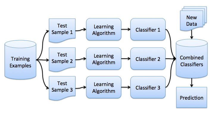
Now that you've gotten the bootstrap idea, we can move on to bagging. In a problem of regression, by averaging the individual responses, bagging reduces the root mean square error by a factor M, the number of regressors.
From our previous lesson, let's recall the components that make up the total out-of-sample error:
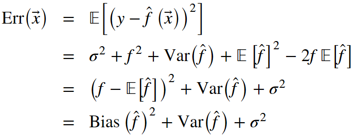
Bagging reduces the variance of a classifier by decreasing the error difference when we train the model on different datasets. In other words, bagging prevents overfitting. The effectiveness of bagging comes from the fact that the individual models are quite different due to different training data and their errors cancel each other out when voting. Also, outliers are likely omitted in some of the training starter samples.
The scikit-learn library supports bagging with the BaggingRegressor and BaggingClassifier meta-estimators. You can use most algorithms as a base.
Let's take a look at how bagging works in practice and compare it with the decision tree. For this we will use an example from the sklearn documentation.
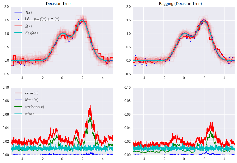
The error for the decision tree:
0.0255 = 0.0003 (bias²)+ 0.0152 (variance) + 0.0098 (σ²)
The error when using bagging:
0.0196 = 0.0004 (bias²) + 0.0092 (variance) + 0.0098 (σ²)
As you can see from the graph above, the error variance is much lower for bagging. Remember that we have already proven this theoretically.
Bagging is efficient on small datasets. Removing even a small part of the training data leads to the construction of significantly different base classifiers. If you have a large data set, you will generate bootstrap samples of a much smaller size.
The example above is unlikely to apply to real work. This is because we made the strong assumption that our individual errors are uncorrelated. More often than not, this is far too optimistic for real-world applications. When this assumption is false, the reduction in error will not be as great. In subsequent lectures, we will discuss some more sophisticated ensemble methods, which allow for more accurate predictions in real-world problems.
Out-of-bag error
In the future, in the case of random forest, it is not necessary to use cross-validation or exclusion samples to obtain an unbiased error estimate. Why? Because, in ensemble techniques, error estimation takes place internally.
Random trees are constructed using different bootstrap samples from the original dataset. About 37 % of the inputs are excluded from a particular bootstrap sample and are not used in the construction of the K-th tree.
Let's see how Out-of-Bag (or OOBE) error estimation works:
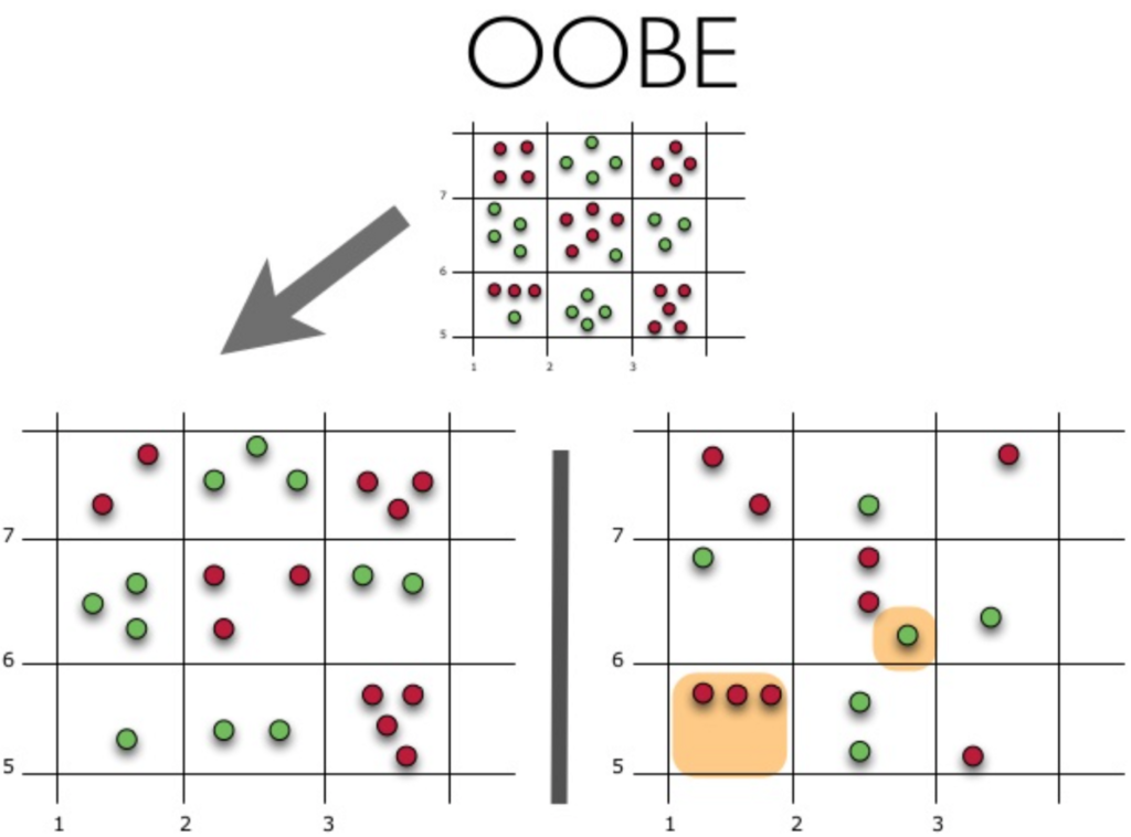
The upper part of the figure above represents our original dataset. We've split it into practice (left) and test (right) sets. In the image on the left, we draw a grid that neatly divides our dataset by classes. Now we use the same grid to estimate the share of correct answers on our test set. We can see that our classifier gave incorrect answers in these 4 cases which were not used during training (left). Therefore, the precision of our classifier is 11/15*100 % = 73.33 %.
To sum up, each algorithm base is trained on ~63 % of the original examples. It can be validated on the remaining ~37%. The Out-of-Bag estimate is nothing more than the average estimate of the base algorithms over the ~37 % of inputs that have not been trained.
Random forest
Leo Breiman succeeded in applying the bootstrap not only in statistics but also in machine learning. Together with Adel Cutler, he extended and improved the Random Forest algorithm proposed by Tin Kam Ho. They combined the construction of uncorrelated trees using CART, bagging and the random subspace method.
Decision trees are a good choice for the basic classifier in bagging because they are quite sophisticated and can achieve zero classification errors on any sample. The random subspace method reduces the correlation between the shafts and thus avoids overfitting. With bagging, the core algorithms are trained on different random subsets of the original feature set.
The following algorithm builds a set of models using the random subspace method:
- Suppose the number of instances is equal to n and the number of dimensions of the entity is equal to d.
- Choose M as the number of individual models in the set.
- For each model m, choose the number of features dm < d. As a general rule, the same dm value is used for all models.
- For each model m, create a training set by selecting dm features at random from the feature set d.
- Train each model.
- Apply the resulting ensemble model to a new input by combining the results of all models of M. You can use either majority voting or posterior probability aggregation.
The algorithm is as follows:

The final classifier is the mean of the trees.
For classification problems, it is advisable to set m equal to the square root of d. For regression problems, we usually take m = d/3, where d is the number of features. It is recommended to build each tree until all its leaves contain only 1 instance for classification and 5 instances for regression.
You can think of Random Forest as a clustering of decision trees with the changing selection of a random subset of features with each split.
Comparison
Here are the results for the three algorithms:
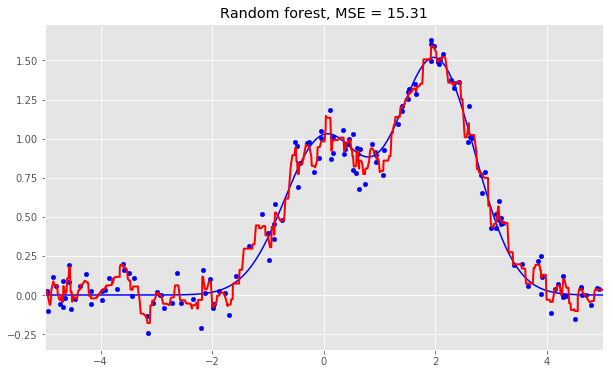
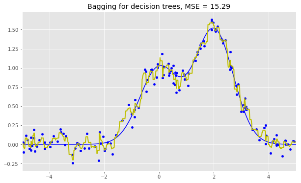

As we can see from our graphs and the MSE values above, a Random Forest of 10 trees achieves a better result than a single decision tree and is comparable to bagging with 10 trees. The main difference between Random Forests and bagging is that, in a Random Forest, the best feature for a split is selected from a random subset of the available features while, in bagging, all features are considered for the next best split.
We can also look at the benefits of random forests and classification problems.


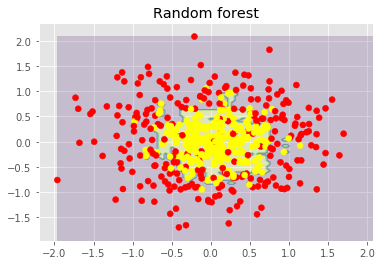
The figures above show that the decision boundary of the decision tree is quite irregular and has many sharp angles that suggest overfitting and poor ability to generalize. We would struggle to make reliable predictions on new test data. In contrast, the bagging algorithm has a rather smooth boundary and shows no obvious signs of overfitting.
Now let's look at some parameters that can help us increase the accuracy of the model.
Parameters to increase accuracy
The scikit-learn library implements random forests by providing two estimators: RandomForestClassifier and RandomForestRegressor.
Below are the parameters we need to pay attention to when building a new model:
- n_estimators is the number of trees in the forest;
- criterion is the function used to measure the quality of a split;
- max_features is the number of features to consider when finding the best distribution;
- min_samples_leaf is the minimum number of samples required to be at a leaf node;
- max_depth is the maximum depth of the tree.
The most important fact about random forests is that its accuracy does not decrease when we add trees, so the number of trees is not a hyperparameter of complexity unlike max_depth and min_samples_leaf. This means you can tune the hyperparameters with, say, 10 trees, then increase the number of trees up to 500 and be sure that the accuracy will only improve.
Extremely random trees use a greater degree of randomization to the choice of cutpoint when splitting a tree node. As in Random Forests, a random subset of features is used. But, instead of searching for optimal thresholds, their values are randomly selected for each possible feature, and the best among these randomly generated thresholds is used as the best rule to split the node. This usually compensates for a slight reduction in model variance with a slight increase in bias.
In the scikit-learn library, there are 2 extremely random tree implementations: ExtraTreesClassifier and ExtraTreesRegressor.
This method should be used if you have overdone it with random forests or gradient boosting.
Conclusion on the random forest
Advantages:
- High prediction accuracy; will perform better than linear algorithms in most problems; the precision is comparable to that of boosting;
- Robust to outliers, thanks to random sampling;
- Insensitive to feature scaling as well as any other monotonic transformation due to random subspace selection;
- Doesn't require fine-tuning of settings, works quite well out of the box. With tuning, an accuracy gain of 0.5 to 3 % can be achieved, depending on the problem tuning and data;
- Effective for datasets with a large number of features and classes;
- Handles both continuous and discrete variables;
- Rarely oversized. In practice, an increase in the number of trees almost always improves the composition. But, after reaching a certain number of trees, the learning curve is very close to the asymptote;
- There are methods developed to estimate the importance of features;
- Works well with missing data and maintains good levels of precision even when a large portion of the data is missing;
- Provides means to weight classes over the dataset as well as for each sample tree;
- Under the hood, calculates proximities between pairs of instances which can then be used in clustering, outlier detection, or interesting data representations;
- The above functionality and properties can be extended to unlabeled data to allow unsupervised grouping, data visualization and detection of outliers;
- Easily parallelized and highly scalable.
The inconvenients:
- Compared to a single decision tree, the output of Random Forest is more difficult to interpret.
- There are no formal p-values for estimating feature importance.
- Performs less well than linear methods in the case of sparse data: text entries, bag of words, etc. ;
- Unlike linear regression, Random Forest is unable to extrapolate. But this can also be seen as an advantage because outliers do not cause outliers in random forests;
- Prone to overfitting in some problems, especially when dealing with noisy data;
- In the case of categorical variables with varying numbers of levels, random forests favor variables with a larger number of levels. The tree structure will adapt more to multi-level functionality, as it becomes more precise;
- If a dataset contains groups of correlated features with similar importance for the predicted classes, preference will be given to smaller groups;
- The resulting model is large and requires a lot of RAM.
