This page shows several examples on the use cases of the different means, in particular the geometric mean and the harmonic mean.

Contents
ToggleArithmetic average
The arithmetic mean is named appropriately: we find it by adding all the numbers in the dataset, then dividing by the number of numbers in the dataset (to bring the sum down to the scale of the numbers original).
3 + 8 + 10 = 21
21 ÷ 3 = 7
Arithmetic mean = 7
Notice, what we're basically saying here is: if every number in our dataset was the same number, what number would it have to be to have the same sum as our actual dataset?
But there's nothing particularly special about the addition. It's just a fairly simple mathematical operation. The arithmetic mean works well to produce an "average" number of a data set when there is an additive relationship between the numbers.
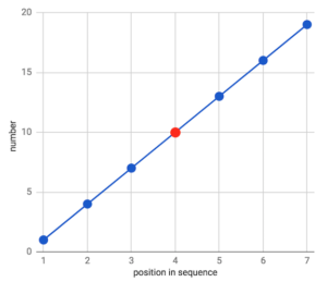
Such a relationship is often called "linear", because when graphed in ascending or descending order, numbers tend to fall on or around a straight line. A simple idealized example would be a dataset where each number is produced by adding 3 to the previous number:
1, 4, 7, 10, 13, 16, 19...

The arithmetic mean therefore gives us a perfectly reasonable median value:
(1 + 4 + 7 + 10 + 13 + 16 + 19) ÷ 7 = 10

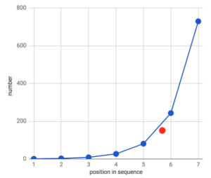
But not all data sets are better described by this linear regression. Some have a multiplicative or exponential relationship, for example if we multiply each consecutive number by 3 rather than adding by 3 as we did above:
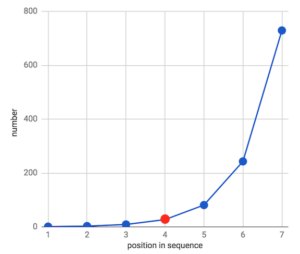
1, 3, 9, 27, 81, 243, 729…
This produces what is called a geometric series. When drawn in order, these numbers look more like a curve than a straight line.
In this situation, the arithmetic mean is ill-suited to produce an "average" number to summarize this data.
(1 + 3 + 9 + 27 + 81 + 243 + 729) ÷ 7 = 156.1

156 is not particularly close to most numbers in our data set. In fact, it's more than 5x the median (middle number), which is 27.
What to do in this case ?
The geometric mean
Since the relationship is multiplicative, to find the geometric mean we multiply rather than add all the numbers. Then, to scale the product to the range of the dataset, we need to take the root of the item count, rather than just dividing.
Thus, the geometric mean of our dataset is:
1 * 3 * 9 * 27 * 81 * 243 * 729 = 10,460,353,203
7th root of 10,460,353,203 = 27
geometric mean = 27

In this case, our geometric mean closely resembles the median value of our data set. In fact, it equals the median.
The geometric mean will not always equal the median, only in cases where there is an exact and consistent multiplicative relationship between all the numbers (for example, multiplying each previous number by 3, as we have done).
Real-world datasets rarely contain such exact relationships, but for those that approximate this type of multiplicative relationship, the geometric mean will yield a closer "median number" than the arithmetic mean.
Example of geometric mean
Suppose we have 100,000 $ which generates a variable interest rate every year for 5 years:
annual interest rates: 1%, 9%, 6%, 2%, 15%
We'd like to take a shortcut to find our average annual interest rate, and therefore our total amount of money after 5 years, so we try to "average" these rates:
(.01 + .09 + .06 + .02 + .15) ÷ 5 = .066 = 6.6%
Next, we insert this average percentage into a compound interest formula:
Total interest earned = $100,000 * (1.066⁵ - 1) = $37,653.11
Interest + principal = $37,653.11 + 100,000 = $137,653.11
final total = $137,653.11
Let's compare the results:
Year 1: 100,000 + (100,000 * .01) = 100,000 * 1.01 = $101,000Year 2: 101,000 * 1.09 = $110,090Year 3: 110,090 * 1.06 = $116,695.40Year 4: 116,695.40 * 1.02 = $119,029.31Year 5: 119,029.31 * 1.15 = $136,883.70Actual final total = $136,883.70
Our shortcut overestimated our actual earnings by nearly 1,000 $.
We made a common mistake: we applied an additive operation to a multiplicative process and got an inaccurate result.
Let's try again with the geometric mean:
1.01 * 1.09 * 1.06 * 1.02 * 1.15 = 1.368837042
5th root of 1.368837042 = 1.064805657
geometric mean = 1.064805657
Plug the geometric mean of interest rates into our compound interest formula:
Total interest earned = $100,000 * (1.0648⁵ - 1) = $36,883.70
Interest + principal = $36,883.70 + 100,000 = $136,883.70
final total = $136,883.70 exactly the same as the long method above
Which corresponds to reality!
Geometric mean and scale change
A cool feature of geometric mean is that you can actually average numbers on completely different scales.
For example, we want to compare the online ratings of two coffeeshops using two different sources. The problem is that source 1 uses a 5 star scale and source 2 uses a 100 point scale:
Coffeeshop A
source 1rating:4.5spring 2rating:68Coffeeshop B
source 1rating:3spring 2rating:75
If we naively take the arithmetic mean of the raw scores of each coffeeshop:
Coffee shop A =
(4.5 + 68) ÷ 2 = 36.25Coffeeshop B =(3 + 75) ÷ 2 = 39
We would conclude that Coffeeshop B was the winner.
If we knew the numbers a little better, we would know that we need to normalize our values on the same scale before averaging them with the arithmetic mean, to get an accurate result. So we multiply the ratings from Source 1 by 20 to scale them from a 5-star scale to the 100-star scale from Source 2:
Coffeeshop A
4.5 * 20 = 90
(90 + 68) ÷ 2 = 79
Coffeeshop B
3 * 20 = 60
(60 + 75) ÷ 2 = 67.5
So we find that Coffeeshop A is the true winner, unlike the naive application of the arithmetic mean above.
The geometric mean, however, allows us to reach the same conclusion without having to worry about scale or units of measurement:
Coffeeshop A =
square root of (4.5 * 68) = 17.5Coffeeshop B =square root of (3 * 75) = 15
And There you go !
The arithmetic mean is dominated by larger scale numbers, which makes us think that Coffeeshop B is the top rated store. This is because the arithmetic mean expects an additive relationship between numbers and ignores scales and proportions. Hence the need to put the numbers on the same scale before applying the arithmetic mean.
The geometric mean, on the other hand, can easily handle varying proportions, due to its multiplicative nature. This is an extremely useful property, but notice what we're losing: we have no interpretable scale at all. The geometric mean is effectively unitless in such situations.
And the harmonic mean?
While the arithmetic mean requires addition and the geometric mean uses multiplication, the harmonic mean uses inverses.
As you may recall, the inverse of a number n is simply 1/n. (for example, the reciprocal of 5 is 1/5). For numbers that are already fractions, this means you can simply "flip" the numerator and denominator: inverse of 4/5 = 5/4. This is true because 1 divided by a fraction gives the inverse of that fraction, e.g. 1 ÷ (4/5) = 5/4.
Thus, the harmonic mean can be described in words: the inverse of the arithmetic mean of the inverses of the data set.
It's really just a few simple steps:
1. Take the reciprocal of all numbers in the dataset
2. Find the arithmetic mean of those reciprocals
3. Take the reciprocal of that number
In mathematical notation, this looks like:

The harmonic mean of 1, 4 and 4 is 2.
Note: Because 0 has no inverse (nothing can be multiplied by 0 for = 1), the harmonic mean also cannot handle data sets that contain 0s, like the geometric mean.
But what is that for ?
Example of harmonic mean
Again, similar to using the geometric mean as the counterpart of the arithmetic mean for multiplicative or nonlinear relationships, the harmonic mean helps us find multiplicative/dividing relationships between fractions without worrying about common denominators.
As such, the harmonic mean naturally accepts another multiplication/division layer on top of the geometric mean. It is therefore useful when dealing with data sets of rates or ratios (i.e. fractions) over different lengths or time periods.
The canonical example of using harmonic means in the real world involves traveling through physical space at different speeds, i.e. speeds.
Consider a trip to the grocery store and back:
- On the way, you drove 30 mph the whole way
- On the way back, traffic was slow and you drove 16 km/h the whole way
- You took the same route and covered the same amount of ground (5 miles) each way.
What was your average speed for the entire duration of this trip?
Again, we could naively apply the arithmetic mean to 30 mph & 10 mph, and proudly declare "20 mph!" »
Since you traveled faster in one direction, you traveled that 8 km faster and spent less time traveling at that speed, so your average travel speed over the entire duration of your trip n It's not the midpoint between 30 mph and 10 mph, it should be closer to 10 mph because you've spent more time riding at that speed.
In order to properly apply the arithmetic mean here, we need to determine the time spent traveling at each fare and then weight our arithmetic mean calculation appropriately:
Trip There: (at 30 mph)
30 miles per 60 mins = 1 mile every 2 minutes = 1/2 mile every minute
5 miles at 1/2 mile per minute = 5 ÷ 1/2 = 10 minutes
"Trip There" time = 10 minutes
Trip Back: (at 10 mph)
10 miles per 60 mins = 1 mile every 6 minutes = 1/6 mile every minute
5 miles at 1/6 mile per minute = 5 ÷ 1/6 = 30 minutes
"Trip Back" time = 30 minutes
Total trip time = 10 + 30 = 40 minutes
“Trip There” % of total trip = 10 / 40 minutes = .25 = 25%
“Trip Back” % of total trip = 30 / 40 minutes = .75 = 75%
Weighted Arithmetic Mean = (30mph * .25)+(10mph * .75) = 7.5 + 7.5 = 15
Average rate of travel = 15 mph
So we see that our true average rate of travel was 15 mph, which is 5 mph (or 25 %) less than our naïve claim of 20 mph using an unweighted arithmetic mean.
Let's try again using the harmonic mean.
Harmonic mean of 30 and 10 = ...
Arithmetic mean of reciprocals = 1/30 + 1/10 = 4/30 ÷ 2 = 4/60 = 1/15
Reciprocal of arithmetic mean = 1 ÷ 1/15 = 15/1 = 15
And There you go !
