Branch and bound

Contents

The Branch and bound algorithm is an "intelligent" enumeration of the tree of possible solutions.

As its name suggests, the algorithm has two times:

separation: to separate a set of solutions into subsets;
evaluation: evaluate the solutions of a subset by increasing the value of the best solution of this subset.

The Branch and bound algorithm (Separation and evaluation) proposes to go through the tree structure of possible solutions by evaluating each subset of solutions. It keeps in memory the value of the best solution f (s) found so far. When the evaluation of a subset gives a value lower than f (s), the algorithm deems useless to explore it directly after.

The Branch and bound algorithm is often used instead of the dynamic programming. The evaluation is often the objective function with relaxed constraints (by decreasing number) according to the depth.

The separation

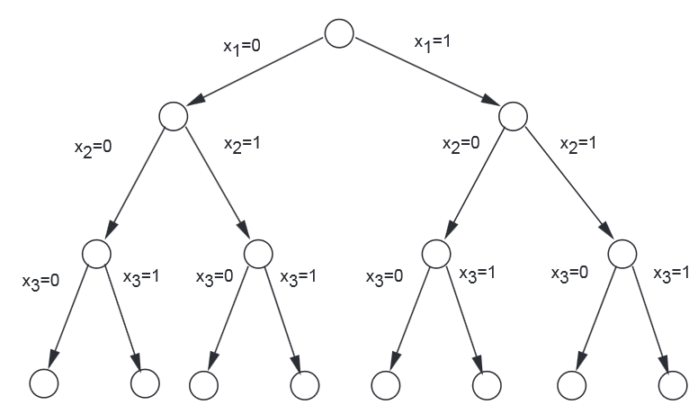
Branch and bound begins with separation. The set of solutions is separated by fixing the value of one or more variables of the problem. Suppose a problem with three variables, the complete tree of separation in ascending order of the variables is as follows:

There are two exploration techniques, linked to the paths of a tree. Breadth first consists of favoring the widening of possibilities by increasing depth, there is no backtracking. Depth first favors the widening of possibilities by visiting the deepest leaves. The advantage is to quickly provide “good” solutions and to eliminate sub-optimal branches.

Evaluation

Branch and bound takes turns evaluating each separation. The root of the tree is an admissible solution which will serve as a reference. We thus obtain a solution giving a value z increasing the optimal solution.

For the subsets of solutions to be tested, noted S_i, we are looking for a lower bound of the objective function in each subset. We therefore have evaluation (S_i) ≤min_{(x∈S_i)} f (x). For the case of a maximum, we are looking for an upper bound evaluation (S_i) ≥max_{(x∈S_i)} f (x).

Assessment is often performed on the initial problem after relaxation. A relaxation makes it possible to pass from complex constraints to linear constraints or of which the dual is simple. For example, integrity relaxation allows working with real variables instead of whole variables.

Once the assessment has been carried out, two cases are possible:

If evaluation (S_i) ≥z, then S_i does not contain any optimal solution, it is not useful to explore in detail the subset S_i.
If evaluation (S_i) <z, alors on teste l’admissibilité de la solution d’évaluation. Si elle est admissible, on actualise z, sinon on continue l’exploration jusqu’à l’obtention d’une des conditions précédentes.

Example: backpack problem

A cargo plane has a cargo capacity of 18 volume units. He must transport containers of goods in such a way as to maximize the total value of his cargo. The available containers are in unlimited quantity for each type:

Type A container, value 6, volume 2;
Type B container, value 8, volume 3;
Type C container, value 13, volume 4;
Type D container, value 17, volume 5;
Type E container, value 20, volume 7.

At first, we will solve the problem using a algorithm gluttonous. Then we will determine the optimal solution by a Branch&Bound procedure.

The mathematical modeling of the problem is the following system: max z=6*x_TO+ 8 * x_B+ 13 * x_VS+ 17 * x_D+ 20 * x_E under 2 * x_TO+ 3 * x_B+ 4 * x_VS+ 5 * x_D+ 7 * x_E≤18 with x_i the integer number of type i containers.

The initial solution is carried out by the greedy algorithm of the best value / volume ratio. We get the solution vector (1,0,0,3,0) with z = 57. x_D being the largest, we will perform the separation on this criterion. We will obtain 4 branches for respectively x_D= 3, 2, 1 and 0:

x_D=3. We solve the linear program relaxed which gives x_VS= 3/4 and z = 60.75. It is an inadmissible solution therefore one separates compared to x_TO :
- x_TO=1. the linear problem relaxed gives x_VS= 1/4 and z = 60.25. This is an unacceptable solution. It is no longer possible to separate because there are no more x_i> 0. The closest whole solution comes down to our starting approximate solution.
- x_TO= 0. The relaxed linear problem gives x_B= 1. The solution is admissible and gives z = 59. We update z.
x_D= 2. We solve the relaxed linear program which gives x_VS= 2 and z = 60. It is an admissible solution so we update z.
x_D= 1. We solve the relaxed linear program which gives x_VS= 13/4 and z = 59.25. This bound is lower than z, so we do not visit this branch.
x_D= 0. We solve the relaxed linear program which gives x_VS= 9/2 and z = 58.5. This bound is lower than z, so we do not visit this branch.

The whole area is explored. The optimum z * = 60 was obtained with the solution vector (0,0,2,2,0).