This page presents a detailed corrected exercise of the problem of linear programming solved by the algorithm of branch and bound.

Contents
ToggleBranch and bound step-by-step corrected exercise
A machine shop owner plans to expand by purchasing new machines, presses and lathes. The owner estimated that each purchased press will increase profits by 100 $ per day and each spin will increase profits by 150 $ per day. The number of machines the owner can purchase is limited by the cost of the machines and the floor space available in the workshop. Machine purchase prices and space requirements are as follows.
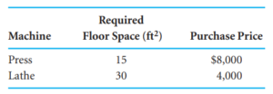
The owner has a budget of 40,000 $ for the purchase of machinery and 200 square feet of floor space available. The owner wants to know how many of each type of machine to buy to maximize the daily increase in profits. Solve this problem.
Solution
The first step is modeling the problem, this is a linear problem as an integer (so the simplex cannot apply).
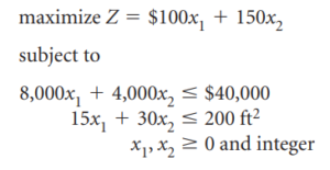
With x_1 the number of presses and x_2 the number of turns.
We start the branch and bound method by first solving the problem as a regular linear programming model with no restrictions on integers (that is, restrictions on integers are relaxed or relaxed). The linear programming model for the problem and the optimal relaxed solution is

The relaxed optimal solution is x_1=2.22 and x_2=5.56 with Z=1055.56.
The branch and bound method uses a diagram consisting of nodes and branches as a framework for the solution process. The first node in the branch and link diagram, shown in Figure C-1, contains the relaxed linear programming solution shown earlier and the rounded solution.
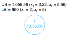
We denote upper bound the result of the relaxed optimal solution, and lower bound the result of the optimal solution as an integer (rounded down).
First connection
Create two constraints (or subsets) to eliminate the fractional part of the value from the solution and see which is farthest from the rounded integer value (i.e. which variable has the largest fractional part in value absolute). The 0.56 part of 5.56 is the largest fractional part; thus, x_2 will be the variable we are going to "plug" into.
In other words, we will create two alternative linear programs taking into account respectively that x_2 must be less than or equal to 5 on the one hand; and x_2 must be greater than or equal to 6 on the other hand.
So we have the following connection:

Let's solve the problem on the left:
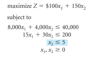
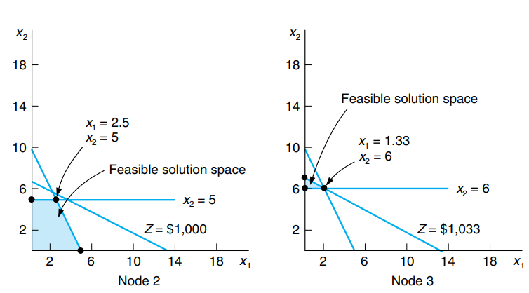
This gives the solution x_1=2.5, x_2=5 and Z=1000.
Let's solve the system on the right:
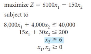
This system has for solution x_1=1.33 and x_2=6, Z=1033.33
From a practical point of view, we cut the definition field with the constraint x_2=6 and have resolved on either side of the constraint the linear system released.
Let's update our graph with the new UB and LB of each system obtained.
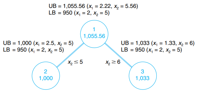
Since we don't have an optimal and feasible integer solution yet, we need to continue branching (i.e., partitioning) the model, either from node 2 or from node 3. A look at Figure reveals that if we branch from node 2, the maximum value that can possibly be reached is 1000 $ (the upper bound).
However, if we start from node 3, a higher maximum value of 1033 $ is possible. Thus, we will branch off from node 3. In general, always branch off from the node with the maximum upper bound.
Second connection
Now the branching steps previously followed at node 1 are repeated at node 3. First, the variable that has the value with the largest fractional part is selected. Since x_2 has an integer value, x_1, with a fractional part of 0.33, is the only variable we can select. Thus, two new constraints are developed from x_1.

Taking node 4, we have the following linear program:

The solution to the problem is x_1=1 and x_2=6.17 with Z=1025.
The second problem is:
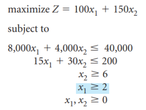
This problem does not admit a solution (first constraint is violated). So we have the following solution graph:
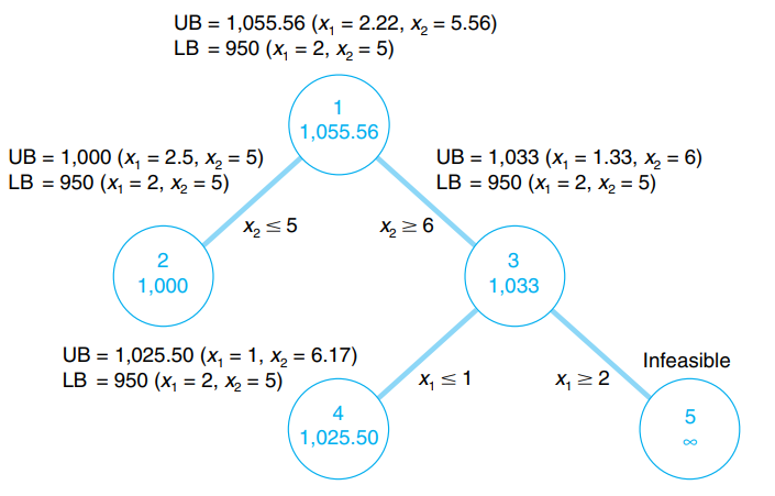
We still don't have an integer solution, so we have to continue the branch and bound algorithm
Third connection
Node 4 has the best UB. Since x_2 is the only variable that is not an integer, we will branch to this variable.
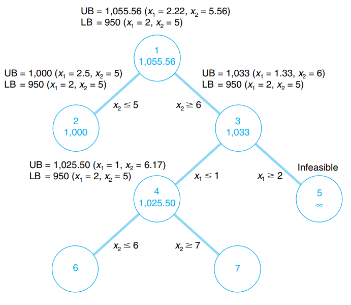
After solving the two linear programs at nodes 6 and 7, we obtain the following results:
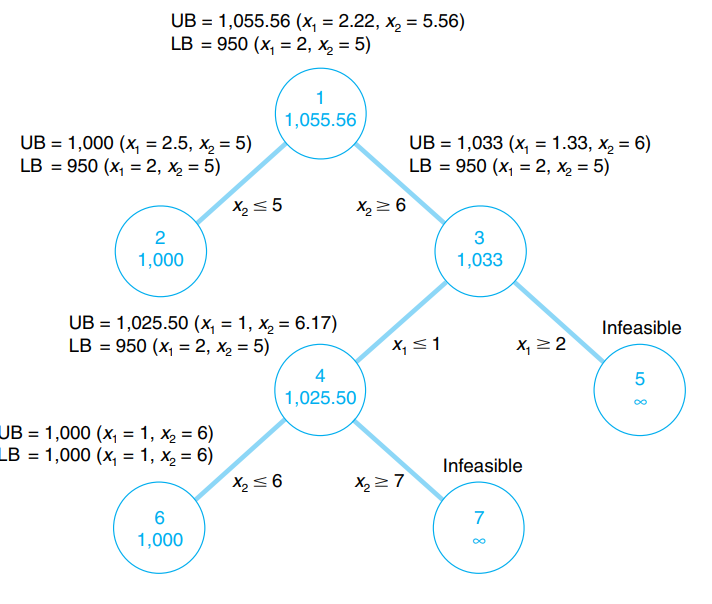
The solution to node 6 corresponds to the criteria of the original problem (ie in whole number). Only the branch at 3 and 4 have a UB higher than node 6, however, the branch that gives node 5 and 7 does not have a feasible solution. We conclude that the optimal solution is found at node 6.
Summary of the method
Here is a summary in English of the method we have just used.
