Mathematical modeling

Mathematical modeling

Mathematical modeling is the basis of all engineering work. Mathematical modeling is characterized by three concepts:

1. The presence of choice, to be made among a finite set (notion that can be compared to the theory of probabilities)
2. A principle of constraints defining the finite set of choices
3. A principle of evaluating the available choices

Mathematical modeling of a problem

The four stages of mathematical modeling of an industrial problem are as follows:

• What are the data of the problem? collect the data of the problem, understand the problem;
• How to model the problem? the three points of thehelp with the decision
  • What decisions do we have to make? select / place objects, define an order or quantity, choose an event, perform a particular operation;
  • What are the constraints of the problem? respect capacities or constraints of precedence;
  • What is the objective sought? maximize profit, minimize costs or quantity;
• What is the complexity of this problem? polynomial, Np, Np-difficult;
• How to solve the problem ? design algorithms (exact vs approximate) giving feasible / optimal solutions, develop alternative or hybrid methods

Depending on the mathematical modeling, the model can also serve as a simulation. It is then possible to see the impact of certain decisions in a context different from that studied (such as the study of the sensitivity of the simplex).

Decision making and mathematical modeling 

Decision making during mathematical modeling involves three major phases followed by the validation phase:

• Collecting information: Examine and identify the problem (variables, functions, values, etc.).
  • Identifying the problem: Identification of organized goals and objectives related to a problem. To determine if a problem exists, identify its symptoms, determine their extent, and define it explicitly. Some problems may arise during data collection and estimation like lack of data, imprecise or inaccurate data, poor estimation, information overload, simulated data, etc.
  • Classification of the problem: The classification of the problem is the placement of a problem in a definable category. This leads to a standardized solution approach.
  • Breakdown of problems: Many complex problems can be divided into subproblems. Some unstructured problems can have very structured subproblems.
• Design: Build a model that represents the system.
  • Understand the problem: Modeling involves the abstraction of the problem in quantitative and / or qualitative forms.
  • A model is built, tested and validated: For a mathematical model, the variables are identified and the relationships between them are established. All models are made up of three basic components: decision variables, uncontrollable variables, and outcome variables. Relationships math bind these components together. In a non-quantitative model, the relationships are symbolic or qualitative.
• Choice: To select a solution to the model.
  • Recommendation of a solution: When the problem is solved, a solution is chosen based on the model. This is recommended for all solutions.
  • Evaluating a solution: Evaluation is possible if the outcome variables give a quantitative solution. A preference relation over the whole solution gives an order: f (a) ⪯ f (b) means that f (b) is better or equal to f (a) where a, b are variables and f (. ) is a mathematical function based on the result variables. b is the best solution iff: f (x) ⪯f (b) for all x in the set of the solution.
• Implementation: Implement software to solve any instance of mathematical modeling.
  • Classic / iterative implementation: Iterative algorithms use repetitive constructions like loops and sometimes additional data structures like stacks to solve given problems.
  • Recursion: a algorithm recursive is an algorithm that refers to itself repeatedly until a condition of termination matches.
  • Logic: a logic algorithm is composed of a logic component and a control component.
  • Deterministic or non-deterministic: deterministic algorithms solve the problem with an exact decision at each step of the algorithm, while non-deterministic algorithms solve the problems by "guessing". A deterministic algorithm is an algorithm which, given a particular input, will always produce the same output.
  • Exact or approximate: While many algorithms reach an exact solution, approximation algorithms seek an approximation that is close to the true solution. When it is not possible to find the best solution in human time, we can look for a solution approximated by less complex algorithms.
  • Serial, parallel or distributed: these implementations depend on the computer architectures, that is to say on the number of processors which can work on a problem at the same time, and on how to break down the whole process into independent processes.
  • Paradigm: Brute-force; Divide and conquer; Dynamic programming; Look for; Randomized; Reduction. Then we need to check the termination, correctness and completeness of the algorithm.
• Validation: To validate the software if it presents a reasonable computation time and a good solution.
  • The complexity of the best case: This is the complexity to solve the problem for the best input of size n.
  • The complexity of the worst case: This is the complexity to solve the problem for the worst entry of size n.
  • Average complexity of cases: It is the complexity to solve the problem on average. This complexity is only defined with respect to a probability distribution on the inputs. For example, if all entries of the same size are assumed to be equally likely to appear, the average complexity of the cases can be defined relative to the uniform distribution over all entries of size n.

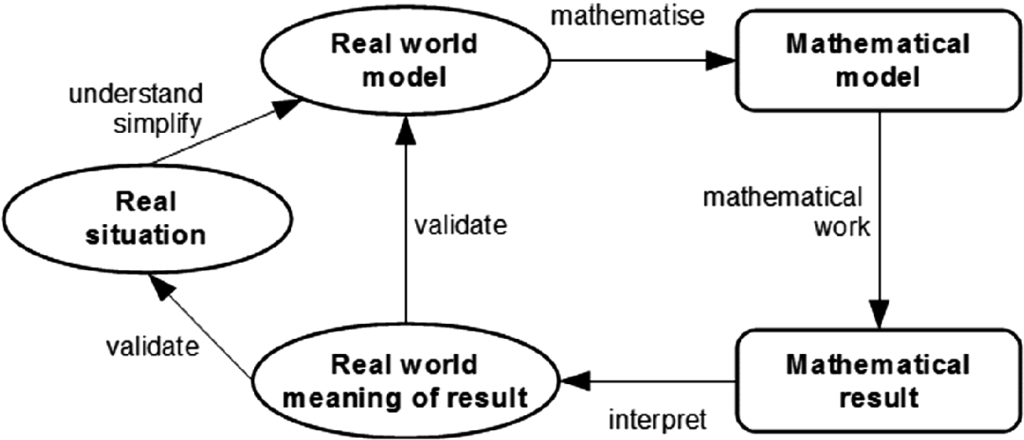
The following diagram shows the mathematical modeling process: