Contents
ToggleCross-validation for time series
In this tutorial, we will explain the principle of cross-validation when learning a time series.

Principle
Time series analysis represents a fundamental approach in the field of statistics and machine learning, aimed at understanding and predicting data patterns that evolve over time. Given the unique characteristics of time series data, including trends, seasonality, and autocorrelation, traditional cross-validation techniques often fail to provide accurate and reliable performance estimates.
To meet these challenges, cross-validation of time series appears to be an essential methodology, adapted to respect the temporal order inherent in the data. This essay explores the intricacies of time series cross-validation, highlighting its meaning, methodology, variations, and practical considerations.
To navigate the river of time, you must respect its current. Time series cross-validation embodies this wisdom, ensuring that our predictions are rooted not only in the data, but in the time stream itself.

The primary goal of time series cross-validation is to evaluate the predictive performance of a model in a way that reflects its future application. This is crucial in various fields, such as finance, meteorology and epidemiology, where decisions are based on forecasts.
Traditional cross-validation methods, which partition data randomly, can disrupt the temporal sequence, leading to overly optimistic performance estimates and models that fail in real-world temporal dynamics. Time series cross-validation preserves chronological order, ensuring that predictions are always based on past information, providing a more realistic assessment of a model's predictive capabilities.
Methodology
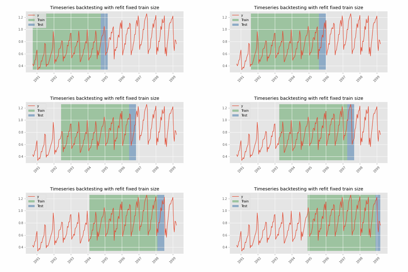
The essence of time series cross-validation lies in its approach of sequentially dividing the dataset. Unlike random partitioning, it systematically expands the training dataset to include more recent observations, while the test set includes observations that immediately follow those in the training set. This procedure is repeated iteratively, each time advancing the cutoff point between the training and testing sets. This approach ensures that the model is validated over different time periods, capturing various temporal dynamics and potential structural changes in the data.
Several variants of time series cross-validation address the specific needs and constraints of time-dependent datasets:
- Single-step forecasting: This is the simplest approach, where the model is trained and validated at single, successive times. It is particularly useful for evaluating model performance in ahead-of-the-box predictions.
- Multi-step forecasting: In multi-step forecasting, the model is tested over multiple future time points in each iteration. This variation is crucial for evaluating model performance over longer horizons, which is essential for planning strategic and decision-making.
- Rolling Origin: Also called “Rolling Forecast Origin” cross-validation, this method involves advancing the starting point of the defined test by one or more periods in each iteration. It allows a complete evaluation of the stability and reliability of the model over time.
- Stretching Window: Unlike the sliding origin technique, varying the stretching window keeps all previous data in the training set, gradually increasing its size. This approach is beneficial for capturing long-term trends and seasonality.
Implementing time series cross-validation requires paying attention to several practical aspects:
- Seasonality and trends: Models should be evaluated across different seasons and trend phases to ensure robustness to temporal changes.
- Stationarity: Ensuring that the time series is stationary, that is, its statistical properties do not change over time, can be crucial for the reliability of cross-validation results.
- Computational efficiency: Time series cross-validation can be computationally intensive, especially for large datasets and complex models. Effective implementation and optimization techniques are essential for practical use.
- Parameter tuning: Nested cross-validation can be used within time series to optimize model parameters, further improving predictive accuracy.
Coded
To demonstrate time series cross-validation with a complete Python code example, we will generate a synthetic time series dataset, implement time series cross-validation, train a simple model, evaluate it using appropriate metrics and visualize the results. This example will use common Python libraries such as pandas, numpy, matplotlib and sklearn.
Let's start with the code:
import numpy ace n.p.
import panda ace pd
from sklearn.linear_model import LinearRegression
from sklearn.metrics import mean_squared_error
import matplotlib.pyplot ace please

# Step 1: Generate Synthetic Dataset
np.random.seed(42)  # For reproducibility
time = np.arange(100)
trend = time * 0.5
seasonality = 10 * np.sin(np.pi * time / 6)
noise = np.random.normal(loc=0, scale=5, size=time.size)
data = trend + seasonality + noise
dates = pd.date_range(start='2020-01-01', periods=time.size, freq='D')
ts_data = pd.Series(data, index=dates)

# Step 2: Time Series Cross-Validation Setup
def time_series_cv(X, y, model, n_splits):
    test_scores = []

    tscv = TimeSeriesSplit(n_splits=n_splits)

    for train_idx, test_idx in tscv.split(X):
        X_train, X_test = X[train_idx], X[test_idx]
        y_train, y_test = y[train_idx], y[test_idx]

        model.fit(X_train, y_train)
        y_pred = model.predict(X_test)
        test_score = mean_squared_error(y_test, y_pred)
        test_scores.append(test_score)

    return test_scores

# Preparing data for modeling
X = time.reshape(-1, 1)
y = data

# Step 3: Model Training
model = LinearRegression()

# Import TimeSeriesSplit
from sklearn.model_selection import TimeSeriesSplit
n_splits = 5
scores = time_series_cv(X, y, model, n_splits=n_splits)

# Step 4: Evaluate Model Performance
print(f'MSE Scores for each split: {scores}')
print(Average MSE: {np.mean(scores)}')

# Step 5: Visualize the Results
plt.figure(figsize=(10, 6))
plt.plot(dates, data, label='True Value', color='blue')
plt.plot(dates, model.predict(X), label='Predicted Value', color='red', linestyle='--')
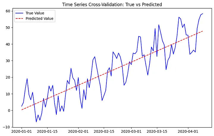
plt.title('Time Series Cross-Validation: True vs. Predicted')
plt.legend()
plt.show()
This code does the following:
- Generates a synthetic time series dataset with trend, seasonality, and noise.
- Implements a rolling forecast origin cross-validation strategy using sklearn's TimeSeriesSplit.
- Trains a linear regression model on time series data.
- Evaluates model performance using the Mean Squared Error (MSE) metric.
- Visualizes actual and predicted values over the time series.
MSE Scores for each split: [113.85938733387366, 125.52615877943208, 70.17575280052887, 74.29515859510016, 78.3146223127321]
Average MSE: 92.43421596433339
