Contents
ToggleDickey-Fuller test
The Dickey-Fuller test is a way to determine if the process (time series) has a unit root.

Bases
We consider the stochastic process of form
![]()
where |φ| ≤ 1 and εi is white noise. If |φ| = 1, we have what we call a unit root. In particular, if φ = 1, we have a random walk (without drift), which is not stationary. In fact, if |φ| = 1, the process is not stationary, whereas if |φ| < 1, the process is stationary. We will not consider the case where |φ| > 1 more since in this case the process is said to be explosive and increases over time.
This process is a first-order autoregressive process, AR(1), which we study in more detail in Autoregressive Processes. We will also see why such processes without a unit root are stationary and why the term "root" is used.
The Dickey-Fuller test is a way to determine whether the above process has a unit root. The approach used is quite simple. First calculate the first difference, i.e.
![]()
that's to say
If we use the delta operator, defined by Δyi = yi – yi-1 and define β = φ – 1, then the equation becomes the equation of regression linear
![]()
where β ≤ 0 and therefore the test for φ is transformed into a test according to which the slope parameter β = 0. Thus, we have a one-sided test (since β cannot be positive) where
H0: β = 0 (equivalent to φ = 1)
H1: β < 0 (equivalent to φ < 1)
Under the alternative hypothesis, if b is the ordinary least squares (OLS) estimate of β, and therefore φ-bar = 1 + b is the ordinary least squares (OLS) estimate of φ, then for sufficiently large n
![]()
or
We can use the usual linear regression approach, except that when the null hypothesis is true, the t coefficient does not follow a normal distribution and therefore we cannot use the usual t test. Instead, this coefficient follows a tau distribution, and so our test is whether the tau statistic τ (which is equivalent to the usual t statistic) is less than τcrit based on a table of critical tau statistic values shown in the Dickey-Fuller table. .
If the calculated tau value is less than the critical value in the critical value table, then we have a significant result; otherwise, we accept the null hypothesis that there is a unit root and that the time series is not stationary.
There are the following three versions of the Dickey-Fuller test:
Type 0 No constant, no trend Δyi = β1 yi-1 + εi
Type 1 Constant, no trend Δyi = β0 + β1 yi-1 + εi
Type 2 Constant and trend Δyi = β0 + β1 yi-1 + β2 i+ εi
Each version of the test uses a different set of critical values, as shown in the Dickey-Fuller table. It is important to select the correct version of the test for the time series being analyzed. Note that the type 2 test assumes that there is a constant term (which can be significantly equal to zero).
Example
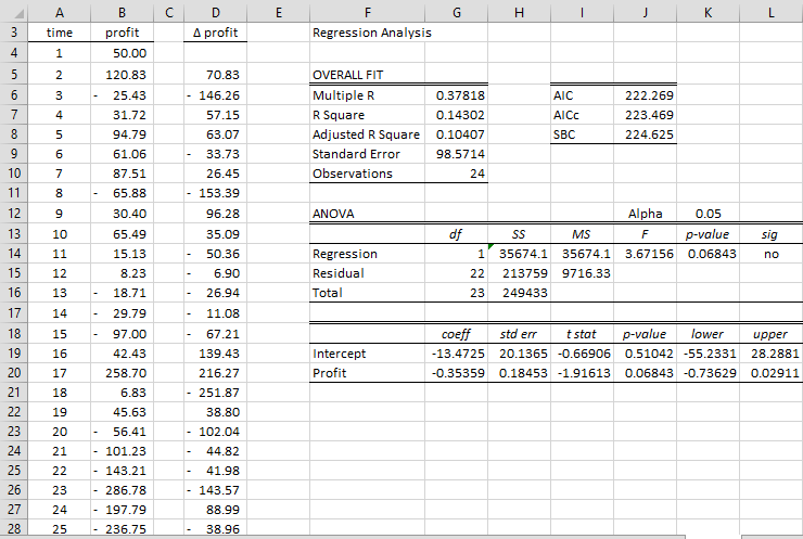
A small player's net daily winnings are listed in column B of Figure 1. Use the Dickey-Fuller test to determine whether the time series is stationary.
We start by assuming that the correct model is type 1, i.e. constant but without trend.

Since we use the regression model
(constant, no trend), we use the tooldata analysis Real Statistics linear regression using range B4:B27 and data range , highlighting the range D5:D28 and pressing Ctrl-D.
The result of the regression analysis is shown on the right side of the figure. In particular, we see that the t statistic (cell I20) for the coefficient β1 is -1.91613. This is the tau statistic. We now look in the Dickey-Fuller table and see that the critical value of tau for a Type 1 test is -2.986 when n = 25 and α = 0.05. Since τcrit = -2.986 < – 1.91613 = τ, we cannot reject the null hypothesis that the time series is not stationary.
Note that the coefficient β1 (cell G20) is negative as expected. If, on the contrary, the coefficient were positive, then we would know that this type of Dickey-Fuller test is inappropriate since β1 = φ – 1 ≤ 0.
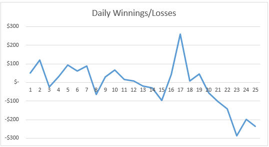
We now show in the figure a plot of the time series values from the previous figure.

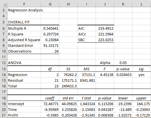
We see an apparent downward trend towards the end of the 25-day period and so it is not surprising that the time series is not stationary. In fact, this leads us to choose the Dickey-Fuller type 2 test (with constant and trend). The result of this test is shown in the figure.

Since we use the regression model
Δyi = β0 + β1i + β2yi-1 + εi
this time we use A4:B27 from Figure 1 as the X data range and D5:D28 as the Y data range. We see in Figure 3 that the t statistic (cell I21) for the coefficient β2 is -2, 91345. We now look in the Dickey-Fuller table and see that the critical value of tau is -3.60269 for a Type 2 test when n = 25 and α = 0.05. Since τcrit = -3.60269 < -2.91345 = τ, we cannot reject the null hypothesis that the time series is not stationary.
