Contents
ToggleDiebold-Mariano test and HLN
Here in detail the Diebold-Mariano test and the measurement of Harvey, Leybourne, and Newbold.

Bases
Suppose we have two forecasts f1, …, fn and g1, …, gn for a time series if y1, …, yn and we want to see which forecast is better, in the sense that it has the best predictive accuracy. The obvious approach is to select the forecast that has the smallest error measure based on one of the error measures described in Forecast Errors. But we need to go further and determine whether this difference is significant (for predictive purposes) or simply due to the specific choice of data values in the sample.
We use the Diebold-Mariano test to determine whether the two predictions are significantly different. Let ei and ri be the residuals of the two forecasts, i.e.
![]()
and is defined as one of the following measures (or other similar measures):
![]()
The time series di is called differential loss. Obviously, the first of these formulas is related to the MSE error statistic and the second is related to the MAE error statistic. We now define

For n > k ≥ 1, we define

As described in the autocorrelation function, γk is the autocovariance at lag k.
For h ≥ 1, define the Diebold-Mariano statistic as follows:

It is generally sufficient to use the value h = n1/3 + 1.
Under the assumption that μ = 0 (the null hypothesis), DM follows a standard normal distribution:
DM ∼ N(0, 1)
There is therefore a significant difference between the forecasts if |DM| > zcrit where zcrit is the two-sided critical value for the standard normal distribution; that's to say.
zcrit = NORM.S.DIST(1–α/2, TRUE)
The key assumption for using the Diebold-Mariano test is that the differential loss time series di is stationary (see Stationary time series).
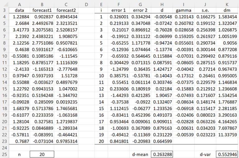
Use the Diebold-Mariano test to determine whether there is a significant difference in the predictions in columns B and C of Figure 1 for the data in column A.

Calculation with Excel
We start by calculating the residuals for the 20 data items based on the two predictions (columns F and G). For example. cell F4 contains the formula =A4-B4 and cell G4 contains =A4-C4. From these values we can calculate the loss differentials in column H. E.g. cell H4 contains =F4^2-G4^2. We can now calculate the mean and variance of the time series di via the formulas =AVERAGE(H4:H23) and =VAR.P(H4:H23), as shown in cells H25 and K25.
The γi values can now be calculated as shown in column I. E.g. cell I4 contains the array formula
=SUMPRODUCT(H5:H$23-H$25,OFFSET(H$4:H$23,0,0,E$23-E4)-H$25)/E$23
Alternatively, cell I4 can be calculated using the formula =ACVF(H$4:H$23,E4), as described in Autocorrelation function. Standard errors (column J) and Diebold-Mariano statistics (column K) can then be calculated. For example. cell J4 contains the formula =SQRT(J25/E23), cell J5 contains =SQRT((J$25+2*SUMPRODUCT(I$4:I4))/E$23) (and the same for the other cells in column J) and cell K4 contains the formula =G$25/J4.
We can read the DM statistical values from column K. For example. the DM statistic for order h = 4 is 1.005199, as shown in cell K7. Note that since h = n1/3 + 1 = 201/3 + 1 = 3.7, h = 4 seems like a good order value to use. Since the p-value = 2*(1-NORM.S.DIST(K7,TRUE)) = 0.3148 > 0.05 = α, we conclude that there is no significant difference between the two predictions.
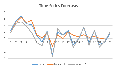
In the figure, we plot both predictions for the data in column A, and so you can judge for yourself whether the graph is consistent with the results of the Diebold-Mariano test.

HLN test
The Diebold-Mariano test tends to reject the null hypothesis too often for small samples. A better test is the Harvey, Leybourne, and Newbold (HLN) test, which is based on the following:
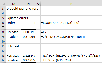
Especially since for example we have a small sample, we use the HLN test as shown in the figure. Once again, we see that there is no significant difference between the forecasts.

