Contents
ToggleCorrected exercises on the dual program and complementary gap
This tutorial offers various corrected exercises on the dual program and the complementary deviation algorithm. The exercises are followed by corrections.

Tutorial
Consider the following linear program:

Solve the linear program.
There are four basic variables for two constraints, it is possible that the problem is not bounded and does not have a solution. Since there are two constraints, the dual will have two variables, it is easy to find a graphical solution to this new linear program.
The dual is as follows:
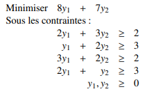
And here is its graphical representation, with a minimum in (1,1) and for objective function 15.
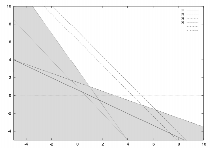
Let's look at the complementary deviations to find a solution of the primal.
- The two variables are non-zero, therefore the two constraints of the primal are saturated (the constraints become equality).
- In the dual, the constraints 1 and 3 are unsaturated for the solution (1,1), this means that the first variable and the third variable of the primal are zero.
So we have the following two equations to solve:
- x2 + 2x4 = 8
- 2x2 + x4 = 7
Which gives for solution (0, 2, 0, 3) and for objective function 15. The solutions of the primal and dual are equal, there is strong duality, it is therefore an optimal solution.
Exercise 1
Solve the following linear program using the dual (graphic resolution + simplex and complementary deviations):
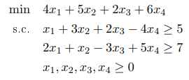
The linear program is in canonical form, so we can calculate the dual without changing the form of the program. The dual is as follows:

with graphic resolution:
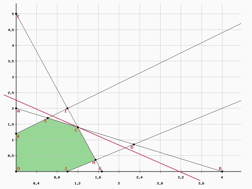
The global optimum is unique and is located at the point (6/5, 7/5) with the objective function Z = 79/5.
For the simplex, the standard form adds a difference variable for each constraint of the linear program. The final table is:
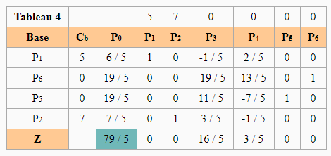
The solution vector of the dual is (6/5, 7/5, 0, 0, 19/5, 19/5) with Z = 79/5. The additional deviations give the following information:
- The third and fourth constraints of the dual are unsaturated, the third and fourth variables of the primal are zero.
- The two basic variables are not zero, the two constraints of the primal are thus saturated.
We must therefore solve the system of equations:
- x1 + 3 x2 = 5
- 2 x1 + x2 = 7
The vector (16/5, 3/5, 0, 0) is solution of the system, with Z = 79/5. There is strong duality so it is about the global optimal of the linear program.
Exercise 2
Consider the following linear program:
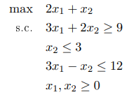
Calculate the optimal solution by graphic resolution. The objective function has for new coefficient (3, 5), to check that the solution found previously is always optimal using the dual and the complementary deviations.
The domain of definition is as follows:
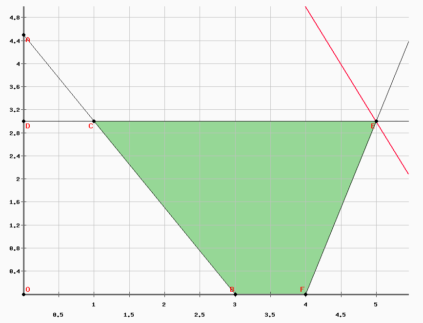
The graphical solution is the vector (5, 3) with Z = 13.
With coefficients of the objective function at (3, 5), we will have Z = 30. Let us check with the complementary deviations if we have a strong duality. The dual program is as follows:

The additional differences are as follows:
- the two basic variables of the primal are non-zero, therefore the two constraints of the dual are saturated
- the first constraint of the primal is unsaturated, so the first variable of the dual is zero.
We must therefore solve the following system:
- 3 x3 = 3
- x2 - x3 = 5
The vector (0, 6, 1) is solution of the system, with Z = 30. There is strong duality therefore (5, 3) is always the optimal solution of the primal program.
Exercise 3
Consider the following linear program:
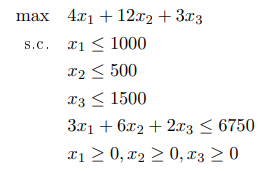
Test the optimality of the solution (250, 500, 1500) using the dual and complementary deviations.
The mathematical modeling turns out to be false, and after checking the vector b of the constraints is (950, 550, 1575, 6900). Using the dual, check whether the solution is admissible and whether it is the optimal solution.
Likewise with the vector (1000, 500, 1500, 9750).
The vector (250, 500, 1500) is an admissible solution because no constraint is violated. The optimal solution has the value Z = 11500. Let us check its optimality by the dual and the complementary deviations. The dual is as follows:

The additional deviations give the following information:
- no base variable of the primal is zero, so the constraints of the dual are saturated
- the first constraint of the primal is not saturated, so the first variable of the dual is zero
This gives the following system:
- 3 X4 = 4
- X2 + 6X4 = 12
- X3 + 2 X4 = 3
With solution vector (0, 4, 1/3, 4/3) with Z = 11500. There is strong duality so this is indeed the optimal solution.
Let us test the optimality again with a primal with the column b = (950, 550, 1575, 6900), only the objective function of the dual changes. The solution is admissible and the additional differences are as follows:
- The three basic variables are non-zero therefore the constraints of the dual are saturated.
- No constraint is saturated, therefore the basic variables of the dual are zero.
No need to solve the dual because the basic variables are all zero (Z = 0), there is no solution to the dual. This means that the solution of the dual is not on an extremum of the domain of definition.
Likewise with the vector b = (1000, 500, 1500, 9750). The solution is admissible and the additional deviations give the following information:
- The three basic variables are non-zero therefore the constraints of the dual are saturated.
- The first and the fourth constraints are unsaturated, therefore the first and the fourth basic variable of the dual are zero.
The system does not admit a solution, therefore the proposed solution is not on an extremum of the domain of definition. Therefore it cannot be the optimum of the linear program.
Exercise 4
When injecting a quantity of electricity into the network, this energy diffuses through the lines offering the least resistance. It is possible to know the lines that will be taken by this energy flow using a linear program.
To do this, the network and the energy flow must be defined:
- the flow starts from a single source and diffuses by the path with the least resistance towards the consumer
- the lines are one-way, the energy flow can only move in the direction of the current already passing through the line
A network is represented in the form of a graph as follows: nodes are substations and arcs representing lines, node 1 is the origin of the energy source, node 7 is the destination of the energy flow.
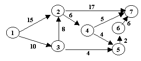
The variables are:
- for each line, a variable between 0 and 1 gives the percentage of use of the line.
The objective function is as follows:
- we try to minimize the total cost, that is to say the sum of the percentages of use of the lines multiplied by the cost of the line.
The constraints are as follows:
- for the original node, the sum of the variables of the outgoing arcs minus the sum of the variables of the incoming arcs is equal to 1
- for the arrival node, the sum of the variables of the incoming arcs minus the sum of the variables of the outgoing arcs is equal to 1
- for the other nodes, the sum of the variables of the outgoing arcs minus the sum of the variables of the incoming arcs is equal to 0.
Represent the linear program of the previous graph, calculate the dual program and solve it using Excel. Deduce the result of the Primal program, note that an equation system can be solved in Excel by the command {= PRODUCTMAT (INVERSEMAT (System); Target vector)} where the coefficients are given in matrix form.
For example :

The linear program representing the shortest path problem is as follows:

The following Excel program gives the solutions of the Primal in Green and the solutions of the Dual in Red (the constraints of the Primal are in line while the constraints of the Dual are in column), note that the equality constraints of the Primal make that the variables of the dual are on the set of reals:

The constraints 4, 5, 7, 8 of the dual are unsaturated, therefore the variables 4, 5, 7, 8 of the primal are zero. We must therefore solve the following system:

This system can be solved very simply without Excel and the answer is the vector (0, 1, 0, 0, 0, 1, 0, 0, 1, 1) and Z = 22. There is strong duality so it is an optimal solution. By representing the arcs used by the energy flow in red, this gives the following diffusion graph:

Exercise 5
An energy island (local network cut off from the global network) has two energy sources and three consumer villages. Plant 1 produces 550 MWh and plant 2 produces 350 MWh. Village 1 requires 400 MWh, village 2 requires 300 MWh and village 3 requires 200 MWh. For each MWh passing through a network line, the cost in euros is as shown in the graph below:

A solution exists if the quantity available is greater than or equal to the quantity requested
- Express the problem of minimizing the cost of energy transit from producers to consumers, explain the objective function and the constraints
- Express the problem of maximizing the profit of energy transit (point of view of the network manager).
- Solve one problem and find a solution for the other using the complementary deviations.
There are 900 quantity available and as many requests, so there is a possible solution. The variables are:
- for each row, X represents the quantity passing through the row.
The objective function is as follows:
- minimize the total cost of resources passing through all lines.
The constraints are as follows:
- stock constraints (less than or equal)
- demand constraints (greater than or equal).
The linear program is as follows:
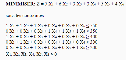
Like the previous exercise, we will solve the primal and the dual on the same Excel sheet:
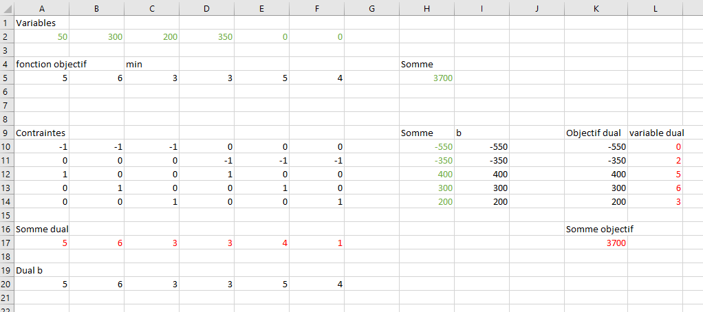
The solution of the dual gives for solution vector (0, 2, 5, 6, 3) with the fifth and sixth unsaturated constraints. It is deduced from this that the first constraint of the primal is not saturated (therefore with a non-zero variation variable) and that the fifth and sixth basic variables are zero. We must therefore solve the following system:

It is possible to find a solution without Excel, this will give the base vector (50, 300, 200, 350, 0, 0) with Z = 3700. By strong duality this is an optimal solution.
