Contents
ToggleTermination and correction
When creating a algorithm, the following three criteria must be taken into account: termination, correction and complexity.
Example
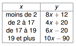
A human being and a dog do not age the same. To determine the human equivalent of the age of a dog under 15kg, we use the table below, where x is the animal's actual age (in years), and y is the human equivalent in term of aging.

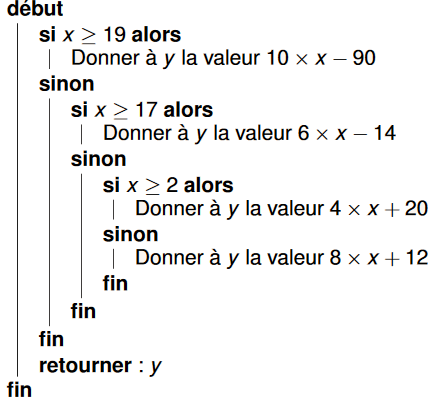
Consider the following algorithm:

Let's check the termination. It is a conditioning suite with elementary calculations inside. Once all the conditions have been verified in order, the algorithm ends.
As regards the correction, the algorithm performs the operations described in the table.
Difficult example
In general, the termination is difficult to verify because we do not always know, a priori, the number of instructions carried out. The correction is complicated when one is in the presence ofhelp with the decision or operations research. It is then necessary to use principles math to prove that the algorithm is correct.
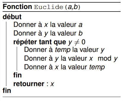
Let us take the example of calculating the gcd in iterative mode.

The algorithm ends if the stop condition of the loop is fulfilled, ie if y is canceled. In the loop, y is replaced by a modulo y remainder. So with each passage, strictly decreases while remaining positive or zero. Therefore, y ends up reaching 0, then we exit the loop. The algorithm ends well after a certain number of iterations.
Initially, x = a and y = b. In the loop, we replace (x, y) by (y, x mod y). We know that pgcd (x, y) = pgcd (y, x mod y). So on each iteration, pgcd (x, y) = pgcd (a, b). At the end of the loop, we have ay = 0, or pgcd (x, 0) = x. By induction we deduce that we return pgcd (a, b). The algorithm correctly calculates the desired gcd.
Tool for termination and correction
We call a loop invariant a property which, if it is true when entering a loop, remains true after each passage through that loop. It is therefore true at the exit of this loop. The loop invariant is analogous to the principle of induction. The demonstration of an adapted loop invariant makes it possible to prove the correctness of an algorithm. For example, pgcd (a, b) = pgcd (x, y) is a loop invariant.
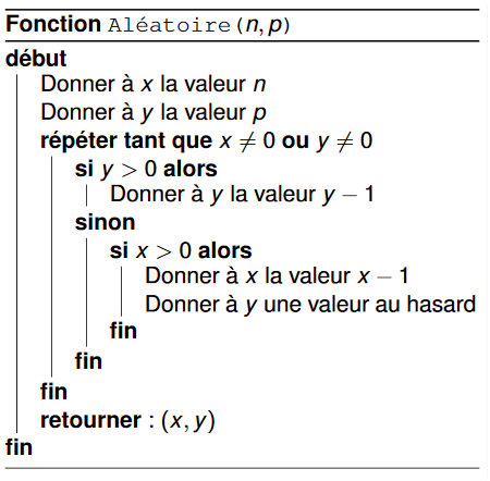
We will take as an example an algorithm with randomness in order to test the notions of termination and correction.

In computer science, randomness attributes a value in a range of values. The pseudo-random is either limited by the size of the container (int, double, etc.) or by the algorithm used (generation of a number modulo a very large number). In the algorithm, we assume that n and p are strictly positive integers. If these have an operation making it negative, then the value of 0 will be automatically assigned.
In the second part of the condition, x decreases while y has a random value (strictly bounded). x therefore tends towards the value 0. In the first part of the condition, y decreases towards 0 from its random value. We therefore conclude that the algorithm decreases y to 0, then decrements x before giving a value to y again.
By induction we conclude that x will tend to 0 after a certain number of iterations, so that the second part will no longer be visited. And y also tends to 0, so we exit the loop. We have therefore proved that the algorithm terminates. It is not useful to talk about correction in this case since we had no specifications to check.
It is noted that some algorithm does not have proof of termination than the famous Syracuse function.
