Contents
ToggleCorrected exercises on sorting algorithms
The following corrected exercises relate to sorting algorithms: Selection sort, insertion sort, bubble sort, cocktail sort, quick sort and merge sort.

Iterative sorts: sort by selection
On an array of n elements (numbered from 0 to n-1), the principle of sorting by selection is as follows:
- search for the smallest element of the array, and exchange it with the element of index 0;
- find the second smallest element of the array, and exchange it with the element of index 1;
- continue in this way until the array is fully sorted.
In pseudo-code, the algorithm is written as follows:
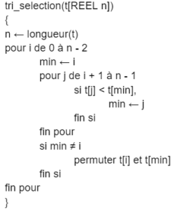
In any case, to sort not elements, sort by selection performs n(n-1)/2 comparisons, therefore in O(n²).
Iterative sorts: insertion sort
Insertion sort is a algorithm classic sorting. Most people naturally use it to sort playing cards.
Insertion sort considers each element of the array and inserts it in the correct place among the already sorted elements. Thus, when an element is considered, the elements which precede it are already sorted, while the elements which follow it are not yet sorted.
To find the place where to insert an element among the previous ones, it must be compared to the latter, and shift them in order to free up a place where to perform the insertion. The offset occupies the space left free by the element considered. In practice, these two actions are performed in one pass, which consists of “raising” the element as it goes until it encounters a smaller element.
Here is an example to better understand the principle on the board [6, 5, 3, 1, 8, 7, 2, 4].
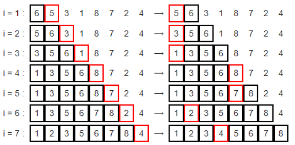
Here is its pseudocode:
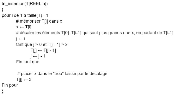
of insertion sort is O(n²) in the worst case and linear in the best case. In the worst case, reached when the array is sorted backwards, the algorithm performs about n²/2 assignments and comparisons; If the array is already sorted, there are n-1 comparisons and at most n assignments.
Iterative sorts: bubble sort
Bubble sort or spread sort is a sorting algorithm. It consists in repeatedly comparing the consecutive elements of an array, and in permuting them when they are badly sorted. It owes its name to the fact that it quickly moves the largest elements to the end of the painting, like air bubbles that would quickly rise to the surface of a liquid.
The algorithm iterates through the array and compares consecutive elements. When two consecutive elements are not in order, they are swapped.
After a first complete scan of the array, the largest element is necessarily at the end of the array, in its final position. Indeed, as soon as the largest element is encountered during the traversal, it is badly sorted in relation to all the following elements, therefore swapped with the next one until reaching the end of the traversal.
After the first run, the largest element being in its final position, it no longer has to be processed. The rest of the painting, however, is still messy. It must therefore be traversed again, stopping at the penultimate element. After this second course, the two largest elements are in their final position. It is therefore necessary to repeat the paths of the table, until the two smallest elements are placed in their final position.
common practice of this sorting consists in interrupting it as soon as a traversal of the elements possibly still in disorder (internal loop) is carried out without permutation. In effect, this means that the entire array is sorted. This optimization requires an additional variable.
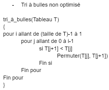

It is possible to put a While instead of the first For. In this case it is necessary to increment i inside the loop and no longer need the break..
For non-optimized sorting, the time complexity is O(n²), with n the size of the array.
For optimized sorting, the number of iterations of the outer loop is between 1 and n. Indeed, we can demonstrate that after the i-th step, the last i elements of the array are in their place. At each iteration, there are exactly n-1 comparisons and at most n-1 permutations.
The worst case (n iterations) is reached when the smallest element is at the end of the array. The complexity is then O(n²). The best case (a single iteration) is reached when the array is already sorted. In this case, the complexity is linear.
Iterative sorting: cocktail sorting
Cocktail sort or shaker sort or two-way bubble sort is a variant of bubble sort1 which is both a sorting algorithm and a comparison sort. The difference between this algorithm and bubble sort is that it performs a sort in each direction on each pass along the list to be sorted.
This sorting algorithm is only slightly more difficult to understand and implement than bubble sort, and it partially solves the turtle problem of bubble sort (turtles are the small items near the end of the original list, which go back only very slowly, one location per iteration, towards their final location).
During the first pass, the first traversal to the right moves elements larger than their immediate neighbor to the right, and, in particular, will move the largest element of the list step by step to its final location at the end of the listing. Then, the second scan to the left will move items smaller than their immediate neighbor to the left, and, in particular, will move the smallest item in the list to its final location at the top of the list. towards the left. Similarly, during the second pass, the second largest element and the second smallest element will in turn join their final location, and so on.
After i passes, the first i elements and the last i elements are in their final location. They therefore no longer need to be verified. It is therefore possible to optimize this algorithm by checking at each pass only the central part of the list not yet sorted definitively. This makes it possible to halve the number of comparisons to be made.
A derivative of the bubble sort is the cocktail sort or shaker sort. This sorting method is based on the following observation: in bubble sort, elements can fast forward to the end of the array, but are only moved to the beginning of the array one position at a time.
The idea of the cocktail sorting is to alternate the direction of the journey. We obtain a sorting a little faster, on the one hand because it requires less comparisons, on the other hand because it reads again the most recent data at the time of the change of direction (they are thus still in the memory cache ). However, the number of permutations to be performed is identical. Thus, the execution time is always proportional to n², therefore mediocre.

The worst-case and best-case complexity in O(.) is the same as bubble sort.
Recursive sorts: quick sort
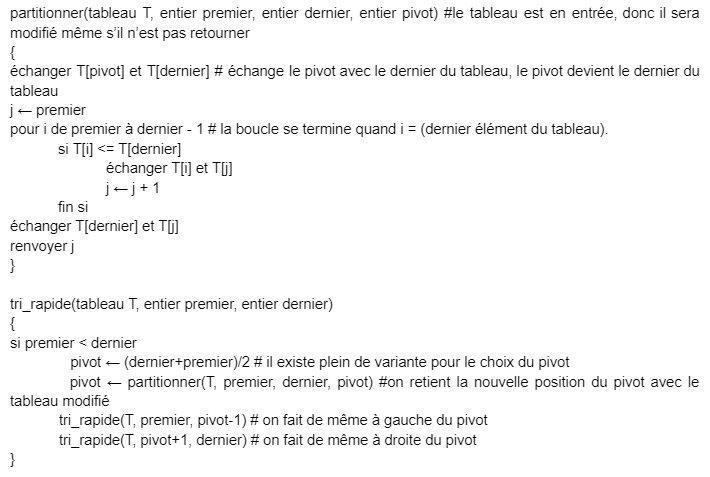
Quicksort is a comparison sorting algorithm, its operation is rather simple to understand and it is widely used on large inputs. Indeed, it has average complexity O(NlogN) and O(N²) in the worst case.
Quick sort uses the principle of divide and conquer, that is to say that we will choose an element of the table (which we call pivot), then we reorganize the initial table into two sub-tables:
- One containing the elements below the pivot.
- The other containing the elements above the pivot.
We continue this process (which we call partitioning, that is to say choosing a pivot and reorganizing the table) until we end up with a table divided into N sub-tables (N being the size of the table), which is so sorted.
Let's take 5, 9, 7, 3, 8 as a sequence of numbers, and sort it in ascending order with the quicksort algorithm:
5, 9, 7, 3, 8 -> we choose the pivot, in our case I choose the middle element, 7.
5, 3 | 7 | 9, 8 -> we cut the painting into three parts, a part with elements below the pivot (5 and 3), the part containing the pivot (7), and a part with the elements above the pivot (9 and 8) . We can already say that we have placed the pivot in its definitive place in the picture, since the other elements are either superior or inferior to it.
5, 3 | 7 | 9, 8 -> we start again by choosing a pivot again for each sub-table created.
3 | 5 | 7 | 8 | 9 -> last step of partitioning, now no sub-arrays contain more than one element, so sorting is over.

Recursive sorts: merge sort
Merge sort is one of the most popular and efficient sorting algorithms. And it's based on the Divide and Conquer paradigm.

Suppose we have to sort an array T. A sub-problem would be to sort a subsection (sub-array) of this array starting at index start and ending at index end, denoted T[start..end ].
If midpoint is the midpoint between start and end, then we can split the subarray T[start..end] into two arrays T[start..mid] and T[mid + 1, end]. In the Conquer step, we try to sort the subnets T[start..middle] and T[middle + 1, end]. If we haven't reached the base case yet (the subarray contains only one element), we again split these two subarrays and try to sort them.
When the conquest stage reaches the base stage and we get two sorted sub-arrays T[start..mid] and T[mid + 1, end] for the array T[start..mid], we combine the results by creating a sorted array T[start..middle] from two sorted subarrays T[start..middle] and T[middle + 1, end].
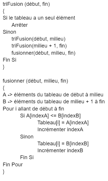
The triMerge function repeatedly splits the array into two halves (two sub-arrays) until we reach a point where we try to perform triMerge on a sub-array of size 1, i.e. start == end.
After that, the merge function kicks in and combines the sorted arrays into a larger array until the whole array is merged. After that, the merge function retrieves the sorted sub-arrays and merges them to gradually sort the whole array.
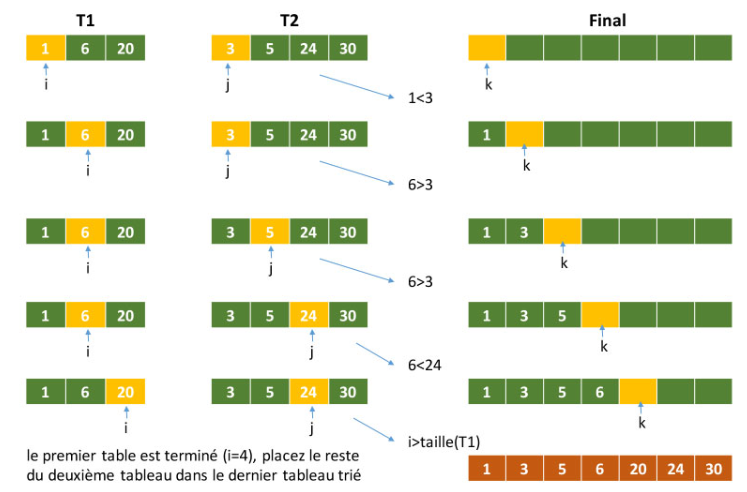
The time complexity of merge sort is O(nLogn) in all 3 cases (worst, average and best) because merge sort always splits the array into two halves and takes linear time to merge two halves.
This pseudo-code is very simplified:
- In the triFusion function, we use recursion to split and then merge our array, and we stop the recursive calls when the subarray we are processing has only one element left.
- The merge function is quite explicit, it allows us to create from two sorted sub-arrays, an array also sorted in linear time.
