Discrete time Markov chains

Difficulty

Easy 25%

Contents

When we are in the presence of a random phenomenon, we notice that the future is dependent only on the present. It is in this condition that one can model the Markov chains in discrete time.

Let (X_not) a sequence of random variables with values in a finite set of J states, X_t= j is the state of the system at time t. We say that X_not is a transition Markov chain if qq is n, qq is i₀,…, I_{n + 1} :

P (X_{(n + 1)}= i_{(n + 1)} | X_not = i_not,…, X₀= i₀) = P (X_{(n + 1)} = i_{(n + 1)} | X_not = i_not)

Such a process is said to be without memory. The value of this probability is denoted by p_{n (n + 1)}.

We notice that X₀ is not fixed by the definition, this law is called the initial law. The vector of the initial probabilities is denoted by π, with π_j= P (S₀= j) with j included in the finite set and the sum of π_j=1.

The vector of transition probabilities is denoted by v_i (p_i0,…, P_ij) with j included in the finite set and the sum of p_ij=1.

The transition probability matrix is the concatenation of the transition probability vectors. All the terms are therefore positive or zero, the sum of the terms on a line is equal to 1. The powers of a transition matrix (or stochastic matrix) are stochastic matrices.

Homogeneous discrete time Markov chains

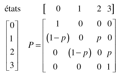
A Markov chain is said to be homogeneous over time if the transition probabilities are not affected by a translation over time. That is, it does not depend on n. The transition probabilities remain stationary over time.

Let's take an example. As long as a player has money, he plays by wagering £ 1. He wins £ 1 with a probability of p and loses his stake with a probability (1-p) with p between 0 and 1. The game ends when he has £ 3.

We can define four states: 0, 1, 2, 3, representing the money he has. The transition matrix is as follows:

The discrete-time Markov chains can have an initial law which is presented in the form of a stochastic vector (the sum is equal to 1). This law represents the distribution at the origin.

Representation of Markov chains in discrete time

The graph associated with a markov process is formed of the points representing the states of the process of the finite set, and of arcs corresponding to the possible transitions p_ij.

Let us denote by Q the transition matrix. A sequence of states (x₁, x₂,. . . , x_m) defines a path of length m going from x₁ to x_m in the graph associated with the homogeneous Markov chain if and only if Q (x₁, x₂) Q (x₃, x₄). . .Q (x_m-1, x_m)> 0.

When we try to simulate the first states of Markov chains in homogeneous discrete time (X_not) of finite state space X = {1,. . . , N} described only by its initial law and its transition matrix Q we can use the following algorithm:

The probability of being in a state j from a state i after n iteration amounts to multiplying the transition matrix Q^not by the initial vector. The answer is then Q^not(i, j).

Reduced graphs of discrete time Markov chains

A state j is accessible from a state i if there is a strictly positive probability of reaching state j from state i in a finite number of transitions. From a point of view of graph theory, j is reachable from a state i if there is a path between i and j.

If state j is accessible from state i and, conversely, state i is accessible from state j, then we say that states i and j communicate. This results in the fact that i and j are on the same circuit.

A reduced graph is a partition of a Markov chain into equivalence classes such that all states of a class communicate with each other.

The equivalence classes are as follows:

a class is said to be transitory if it is possible to leave it, but in this case, the process will never be able to return to it again;
a class is said to be recurrent or persistent if it cannot be left. If a recurrent class is composed of a single state, it is said to be absorbent.

If the partition into equivalence classes induces only one recurrent class, the Markov chain is said to be irreducible. A Markov chain has at least one recurring class.

Example on discrete time Markov chains

We are interested in the development of a natural forest in a temperate region on a plot. Our model has 3 states. State 1 is that of vegetation made up of grasses or other species with a low carbon balance; state 2 corresponds to the presence of shrubs whose rapid development requires maximum sunshine and whose carbon yield will be maximum, and state 3 that of larger trees that can grow in a semi-sunny environment (considered as a forest). If these three states are denoted respectively by h, a, f (for grass, shrubs, forest), the set of possible states for a given point of this plot is the set s={h, a, f}. On the plot, a large number of points distributed on a regular grid are identified on the ground and the state of the vegetation at each of these points is recorded at fixed time intervals. This type of program is called a automaton cellular.

By observing the evolution during an interval of time, one can determine for each state i∈S the proportion of points which passed to the state j∈S, and note p_ij this proportion. If the different proportions thus noted (there are 9) change little from one time interval to the next, we can assume them to be unchanged over time and we can look at the probabilities for any point of passing from the state i in state j for an interval of time. Suppose for example that in this plot, these probabilities are as follows:

If X₀ indicate the state of a point at time t = 0 and X₁ the state of the same point at t = 1, for example we have the probability of passing from the shrub state at t = 0 to the forest state at t = 1 is written P (X₁= f: X₀= a) is equal to 0, 4.

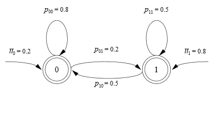
The set of states S and the transition matrix P constitute an example of a Markov chain. We can also represent this Markov chain by the following graph:

In this model, we can thus calculate the probability of any succession of states, called the trajectory of the Markov chain. For example, the probability that at a point on the plot we observe the succession of states (h, h, a, f, f) is calculated as follows:

where π₀ is the probability of being in the state at the initial time t = 0.

Observation of the state in which the various points of the plot are located at the initial time t₀ allows to determine the initial proportions of each of the 3 states. For that, one notes for each point the state in which it is found and one calculates the proportion of points of each of the possible states. We can see each proportion as the probability for a point of the plot to be in one of the states at the initial instant. Thus, if we have for example π₀ = (0.5, 0.25, 0.25), this means that half of the points of the plot are initially in state h, a quarter in state a and a quarter in state f. But we can also interpret this by considering that any state has a 50% chance of being in state h, 25% of being in state a and 25% of being in state f. This is why the proportion of individuals of the studied population located in each of the states,

is called the initial probability law or the initial distribution. When one chooses a modeling by a Markov chain, the objective is often to determine the evolution of the distribution of states over time. For example, if the plot considered above is covered for a third of forest at the initial moment, will this proportion grow, tend towards 100%, on the contrary tend towards zero or approach a value? limit kind of ecological balance?

We will see that if we know the initial distribution we can calculate the distribution at time t = 1, then at time t = 2 and so on. Let us calculate for t = 1:

We deduce that π₁(h) is the dot product of the vector π₀ with the first column of the matrix P. Similarly, we check that π₁(a) is the dot product of the vector with the second column of the matrix P and that π₁(f) is the scalar product of the vector with the third column of the matrix P. We summarize this: π₁= π₀P.